In this post, we will see the main technical ideas in the analysis of the mixing time of evolutionary Markov chains introduced in a previous post. We start by introducing the notion of the expected motion of a stochastic process or a Markov chain. In the case of a finite population evolutionary Markov chain, the expected motion turns out to be a dynamical system which corresponds to the infinite population evolutionary dynamics with the same parameters. Surprisingly, we show that the limit sets of this dynamical system govern the mixing time of the Markov chain. In particular, if the underlying dynamical system has a unique stable fixed point (as in asexual evolution), then the mixing is fast and in the case of multiple stable fixed points (as in sexual evolution), the mixing is slow. Our viewpoint connects evolutionary Markov chains, nature’s algorithms, with stochastic descent methods, popular in machine learning and optimization, and the readers interested in the latter might benefit from our techniques.
A Quick Recap
Let us recall the parameters of the finite population evolutionary Markov chain (denoted by $\mathcal{M}$) we saw last time. At any time step, the state of the Markov chain consists of a population of size $N$ where each individual could be one of $m$ types. The mutation and the fitness matrices are denoted by $Q$ and $A$ respectively. $X^{(t)}$ captures, after normalization by $N,$ the composition of the population is at time $t$. Thus, $X^{(t)}$ is a point in the $m$-dimensional probability simplex $\Delta_m$. Since we assumed that $QA>0$, the Markov chain has a stationary distribution $\pi$ over its state space, denoted by $\Omega \subseteq \Delta_m$; the state space has cardinality roughly $N^m$. Thus, $X^{(t)}$ evolves in $\Delta_m$ and, with time, its distribution converges to $\pi$. Our goal is to bound the time it takes for this distribution to stabilize, i.e., bound the mixing time of $\mathcal{M}$.
The Expected Motion
As a first step towards understanding the mixing time, let us compute the expectation of $X^{(t+1)}$ for a given $X^{(t)}$. This function tells us where we expect to be after one time step given the current state; in this paper we refer to this as the expected motion of this Markov chain (and define it formally for all Markov chains towards the end of this post). An easy calculation shows that, for $\mathcal{M}$,
\[\mathbb{E} \left[ X^{(t+1)} \; \vert \; X^{(t)} \right] = \frac{QA X^{(t)}}{\|QAX^{(t)}\|_1}=: f(X^{(t)}).\]This $f$ is the same function that was introduced in the previous post for the infinite population evolutionary dynamics with the same parameters! Thus, in each time step, the expected motion of the Markov chain is governed by $f$. Surprisingly, something stronger is true: we can prove (see Section 3.2 here) that, given some $X^{(t)},$ the point $X^{(t+1)}$ can be equivalently obtained by taking $N$ i.i.d. samples from $f(X^{(t)})$. In words,
\[f \; \; \mbox{guides} \; \; \mathcal{M}.\]In fact, a moment’s thought tells us that this phenomenon transcends any specific model of evolution. We can fix any dynamical system $g$ over the simplex and define a Markov chain guided by it as follows: If $X^{(t)}$ is the population vector at time $t$, then define $X^{(t+1)}$ as the population vector obtained by taking $N$ i.i.d. (or even correlated) copies from $g(X^{(t)})$. By design, $g$ is the expected motion of this Markov chain.
Evolution on Finite Populations = Noisy Evolution on Infinite Populations
The above observation allows us to view our evolutionary Markov chain as a noisy version of the deterministic, infinite population evolution. A bit more formally, there are implicitly defined random variables $\zeta_{s}^{(t+1)}$ for $1 \leq s \leq N$ and all $t$, such that
\[X^{(t+1)} = f(X^{(t)}) + \frac{1}{N} \sum_{s=1}^N \zeta_s^{(t+1)}.\]Here, $\zeta_s^{(t+1)}$ for $1\leq s \leq N$ is a random vector that corresponds to the error or noise of sample $s$ at the $t$-th time step. Formally, because $f$ is the expected motion of the Markov chain, each $\zeta_s^{(t+1)}$ has expectation $0$ conditioned on $X^{(t)}$. Further, the fact that $f$ guides $\mathcal{M}$ implies that for each $t$, when conditioned on $X^{(t)}$, the vectors $\zeta_{s}^{(t+1)}$ are i.i.d. for $1 \leq s \leq N$. Without conditioning, we cannot say much about the $\zeta_{s}^{(t)}$s. However, since we know that the state space of $\mathcal{M}$ lies in the simplex, we can deduce that $\Vert\zeta_s^{(t)}\Vert \leq 2$. The facts that the expectation of the $\zeta_s^{(t)}$s are zero, they are independent and bounded imply that the variance of each coordinate of $\frac{1}{N} \sum_{s=1}^N \zeta_s^{(t+1)}$ (again conditioned on the past) is roughly $1/N$.
Connections to Stochastic Gradient Descent
Now we draw an analogy of the evolutionary Markov chain to an old idea in optimization, stochastic gradient descent or SGD.
However, we will see crucial differences that require the development of new tools.
Recall that in the SGD setting, one is given a function $F$ and the goal is to find a local minimum of $F.$
The gradient descent method moves from the current point $x^{(t)}$ to a new point $x^{(t+1)}=x^{(t)} - \eta \nabla F(x^{(t)})$ for some rate $\eta$ (which could depend on time $t$).
Since the gradient may not be easy to compute, SGD substitutes the gradient at the current point by an unbiased estimator of the gradient.
Thus, the point at time $t$ becomes a random variable $X^{(t)}$. Since the estimate is unbiased, we may write it as
where the expectation of $\zeta^{(t+1)}$ conditioned on $X^{(t)}$ is zero. Thus, we can write one step of SGD as
\[X^{(t+1)} = \left( X^{(t)} -\eta \nabla F(X^{(t)}) \right) +\eta \cdot \zeta^{(t+1)}.\]Comparing it to our evolutionary Markov chain, it can be shown that $f(x)=\frac{QA x}{\Vert QA x\Vert_1}$ is a gradient system (i.e., $f=\nabla G$ for some function $G$) and we may think of the corresponding $\mathcal M$ as SGD with step-size $\eta=1/N$.
There is a vast literature understanding when SGD converges to the global optimum (for convex $F$) or a local optima (for reasonable non-convex $F$). Why can’t we use techniques developed for SGD to analyze our evolutionary Markov chain? To start with, when the step size does not go to zero with time, $X^{(t)}$ wanders around its domain $\Omega$ and will not converge to a point. In the case when the step size is fixed, typically, the time average of $X^{(t)}$ is used in a hope that it will converge to a local minima of the function. The Ergodic Theorem of Markov chains tells us that the time average will converge to the expectation of a sample drawn from $\pi$, the steady state distribution. This quantity is the same as the zero of $\nabla F$ only when it is a linear function (equivalently $F$ is quadratic); certainly not the case in our setting. Further, the rate of convergence to this expectation is governed by the mixing time of the Markov chain. Thus, there is no getting around proving a bound on the mixing time. Moreover, for biological applications (as described in our previous post), we need to know more than the expectation: we need to obtain samples from the steady state distribution $\pi$. Finally, in several other evolutionary Markov chains of interest, the guiding dynamical system is not a gradient system. Hence, the desired results in the setting of evolution seem beyond the reach of current techniques.
The reason for taking this detour and making the connection to SGD is not only to show that completely different sounding problems and areas might be related, but also that the techniques we develop in analyzing evolutionary Markov chains find use in understanding SGD beyond the quadratic case.
The Landscape of the Expected Motion Governs the Mixing Time
Now we delve into our results and proof ideas. We derive all of the information we need to bound the mixing time of $\mathcal M$ from the the limit sets of $f$ which guides it. Roughly, we show that when the limit set of $f$ consists of a unique stable fixed point (which is akin to convexity) as in asexual evolution, then the mixing is fast and in the case of multiple stable fixed points (which is akin to non-convexity) as in sexual evolution, the mixing is slow.
We saw in our first post that the dynamical system $f(x)=\frac{QAx}{\Vert QAx\Vert_1}$ corresponding to the case of asexual evolution has exactly one fixed point in the simplex, say $ x^\star$, when $QA$ is positive. In fact, $x^\star$ is stable and, no matter where we initiate the dynamical system, it ends up close to $x^\star$ in a small number of iterations (which does not depend on $N$).
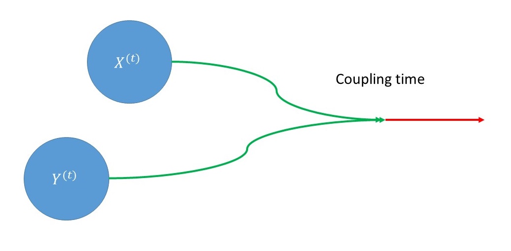
Back to mixing time: a generic technique to bound the mixing time of a Markov chain employs a coupling of two copies of the chain $X^{(t)}$ and $Y^{(t)}$.
A coupling of a Markov chain $\mathcal M$ is a function which takes as input $X^{(t)}$ and $Y^{(t)}$ and outputs $X^{(t+1)}$ and $Y^{(t+1)}$ such that each of $X^{(t+1)}$ and $Y^{(t+1)}$, when considered on their own, is a correct instantiation of one step of $\mathcal M$ from the states $X^{(t)}$ and $Y^{(t)}$ respectively. However, $X^{(t+1)}$ and $Y^{(t+1)}$ are allowed to be arbitrarily correlated.
For example, we could couple $X^{(t)}$ and $Y^{(t)}$ such that if $X^{(t)} = Y^{(t)}$ then $X^{(t+1)}=Y^{(t+1)}$. More generally, we can consider the distance between $X^{(t)}$ and $Y^{(t)}$, and consider a coupling that contracts the distance between them. If this distance is contractive by, say, a factor of $\rho<1$ at every time step, then the number of iterations required to reduce distance below $1/N$ is about $\log_{1/\rho} N$; this roughly upper bounds the mixing time.
The key observation that connects the dynamical system $f$ and our Markov chain is that using the function $f$ we can construct a coupling $\mathcal{C}$ such that for all $x$,$y \in \Omega$,
\[\mathbb{E}_{\mathcal{C}}\left[\|{X}^{(t+1)}-{Y}^{(t+1)}\|_1 \; | \; {X}^{(t)}=x, {Y}^{(t)}=y \right]=\|f(x)-f(y)\|_1.\]Thus, if $ \Vert f(x)-f(y)\Vert_1 < \rho \cdot \Vert x-y\Vert_1 <1$ for some $\rho<1$ and all $x,y \in \Omega$, we would be done. The bad news is that we can show that there are $x,y$ for which $\Vert f(x)-f(y)\Vert_1 > \Vert x-y \Vert_1$ implying that there is no contractive coupling for all $x$ and $y.$
What about when $x$ and $y$ are close to $x^\star$?
In this case, by a first order Taylor approximation of the dynamical system $f$, we can bound the contraction $(\rho)$ by the $1 \rightarrow 1$ norm of the Jacobian of $f$ at $x^\star$. However, this quantity is less than one only when $m=2$, see here. For larger $m$, we have to go back to our intuition from dynamical systems and, using the fact that all trajectories of $f$ converge to $x^\star$, argue that the appropriate norm of the Jacobian of $f^k$ (i.e., $f$ applied $k$ times) is contractive. While there are a few technical challenges, we can use $f^k$ to construct a contractive coupling. We then use concentration to handle the case when $x$,$y$ are not close to $x^\star$, see here for the details. As a consequence, we obtain a mixing time of $O(\log N)$ (suppressing other parameters). Thus, in the world of asexual evolution the steady state can be reached quickly!
Markov Chains Guided by Dynamical Systems - Beyond Uniqueness
Interestingly, this proof does not use any property of $f$ other than that it has a unique fixed point which is stable. However, in many cases, such as sexual evolution (see here for the model of sexual evolution or an equivalent model for how children acquire grammar, see here) and here, the expected motion has multiple fixed points - some stable and some unstable. Such a dynamical system is inherently non-convex - trajectories starting at different points could converge to different points. Further, the presence of unstable fixed points can slow down trajectories and, hence, the mixing time. In this paper, we give a comprehensive treatment about how the landscape of the limit sets determines the mixing time of evolutionary Markov chains. In a nutshell, while the presence of unstable fixed points does not seem to affect the mixing time, the presence of two stable fixed points results in the mixing time being $\exp(N)$!
This result allows us to prove a phase transition in the mixing time for an evolutionary Markov chain with sex where, changing the mutation parameter changes the geometry of the limit sets of the expected motion from multiple stable fixed points to unique stable fixed point.
Evolution on Structured Populations?
A challenging problem left open by our work is to try to estimate the mixing time of evolutionary dynamics on structured populations which arise in ecology. Roughly, this setting extends the evolutionary models discussed thus far by introducing an additional input parameter, a graph on $N$ vertices.
The graph provides structure to the population by locating each individual at a vertex, and, at time $t+1$, a vertex determines its type by sampling with replacement from among its neighbors in the graph at time $t$; see this paper for more details.
The model we discussed so far can be seen as a special case when the underlying graph is the complete graph on $N$ vertices. The difficulty is two fold: now it is no longer sufficient to keep track of the number of each type and also the variance of the noise is no longer $1/N$ - it could be large if a vertex has small degree.
The Expected Motion Revisited
Now we formally define the expected motion of any Markov chain with respect to a function $\phi$ from its state space $\Omega$ to $\mathbb{R}^n$. If $X^{(t)}=x$ is the state of the Markov chain at time $t$ and $X^{(t+1)}$ its state at time $t+1,$ then the expected motion of $\phi$ for the chain at $x$ is
\[\mathbb{E}\left[\phi(X^{(t+1)}) \;| \;X^{(t)} =x \right]\]where the expectation is taken over one step of the chain. Often, and in the application we presented in this post, the state space $\Omega$ already has a geometric structure and is a subset of $\mathbb{R}^n$. In this case, there is a canonical expected motion which corresponds to $\phi$ being just the identity map.
What can the expected motion of a Markov chain tell us about the Markov chain itself?
Of course, without imposing additional structure on the Markov chain or $\phi$, the answer is unlikely to be very interesting. However, the results in this post suggest that thinking of a Markov chain in this way can be quite useful.
To Conclude …
In this post, hopefully, you got a flavor of how techniques from dynamical systems can be used to derive interesting properties of Markov chains and stochastic processes. We also saw that nature’s methods, in the context of evolution, seem quite close to the methods of choice of humans - is this a coincidence? In a future post, we will show another example of this phenomena - the famous iteratively reweighted least squares (IRLS) in sparse recovery turns out to be identical to the dynamics of an organism found in nature - the slime mold.