Word embeddings capture the meaning of a word using a low-dimensional vector and are ubiquitous in natural language processing (NLP). (See my earlier post 1 and post2.) It has always been unclear how to interpret the embedding when the word in question is polysemous, that is, has multiple senses. For example, tie can mean an article of clothing, a drawn sports match, and a physical action.
Polysemy is an important issue in NLP and much work relies upon WordNet, a hand-constructed repository of word senses and their interrelationships. Unfortunately, good WordNets do not exist for most languages, and even the one in English is believed to be rather incomplete. Thus some effort has been spent on methods to find different senses of words.
In this post I will talk about my joint work with Li, Liang, Ma, Risteski which shows that actually word senses are easily accessible in many current word embeddings. This goes against conventional wisdom in NLP, which is that of course, word embeddings do not suffice to capture polysemy since they use a single vector to represent the word, regardless of whether the word has one sense, or a dozen. Our work shows that major senses of the word lie in linear superposition within the embedding, and are extractable using sparse coding.
This post uses embeddings constructed using our method and the wikipedia corpus, but similar techniques also apply (with some loss in precision) to other embeddings described in post 1 such as word2vec, Glove, or even the decades-old PMI embedding.
A surprising experiment
Take the viewpoint –simplistic yet instructive– that a polysemous word like tie is a single lexical token that represents unrelated words tie1, tie2, … Here is a surprising experiment that suggests that the embedding for tie should be approximately a weighted sum of the (hypothethical) embeddings of tie1, tie2, …
Take two random words $w_1, w_2$. Combine them into an artificial polysemous word $w_{new}$ by replacing every occurrence of $w_1$ or $w_2$ in the corpus by $w_{new}.$ Next, compute an embedding for $w_{new}$ using the same embedding method while deleting embeddings for $w_1, w_2$ but preserving the embeddings for all other words. Compare the embedding $v_{w_{new}}$ to linear combinations of $v_{w_1}$ and $v_{w_2}$.
Repeating this experiment with a wide range of values for the ratio $r$ between the frequencies of $w_1$ and $w_2$, we find that $v_{w_{new}}$ lies close to the subspace spanned by $v_{w_1}$ and $v_{w_2}$: the cosine of its angle with the subspace is on average $0.97$ with standard deviation $0.02$. Thus $v_{w_{new}} \approx \alpha v_{w_1} + \beta v_{w_2}$. We find that $\alpha \approx 1$ whereas $\beta \approx 1- c\lg r$ for some constant $c\approx 0.5$. (Note this formula is meaningful when the frequency ratio $r$ is not too large, i.e. when $ r < 10^{1/c} \approx 100$.) Thanks to this logarithm, the infrequent sense is not swamped out in the embedding, even if it is 50 times less frequent than the dominant sense. This is an important reason behind the success of our method for extracting word senses.
This experiment –to which we were led by our theoretical investigations– is very surprising because the embedding is the solution to a complicated, nonconvex optimization, yet it behaves in such a striking linear way. You can read our paper for an intuitive explanation using our theoretical model from post2.
Extracting word senses from embeddings
The above experiment suggests that
\[v_{tie} \approx \alpha_1 \cdot v_{ tie1} + \alpha_2 \cdot v_{tie2} + \alpha_3 \cdot v_{tie3} +\cdots \qquad (1)\]but this alone is insufficient to mathematically pin down the senses, since $v_{tie}$ can be expressed in infinitely many ways as such a combination. To pin down the senses we will interrelate the senses of different words —for example, relate the “article of clothing” sense tie1 with shoe, jacket etc.
The word senses tie1, tie2,.. correspond to “different things being talked about” —in other words, different word distributions occuring around tie. Now remember that our earlier paper described in post2 gives an interpretation of “what’s being talked about”: it is called discourse and it is represented by a unit vector in the embedding space. In particular, the theoretical model of post2 imagines a text corpus as being generated by a random walk on discourse vectors. When the walk is at a discourse $c_t$ at time $t$, it outputs a few words using a loglinear distribution:
\[\Pr[w~\mbox{emitted at time $t$}~|~c_t] \propto \exp(c_t\cdot v_w). \qquad (2)\]One imagines there exists a “clothing” discourse that has high probability of outputting the tie1 sense, and also of outputting related words such as shoe, jacket, etc. Similarly there may be a “games/matches” discourse that has high probability of outputting tie2 as well as team, score etc.
By equation (2) the probability of being output by a discourse is determined by the inner product, so one expects that the vector for “clothing” discourse has high inner product with all of shoe, jacket, tie1 etc., and thus can stand as surrogate for $v_{tie1}$ in expression (1)! This motivates the following global optimization:
Given word vectors in $\Re^d$, totaling about $60,000$ in this case, a sparsity parameter $k$, and an upper bound $m$, find a set of unit vectors $A_1, A_2, \ldots, A_m$ such that \(v_w = \sum_{j=1}^m\alpha_{w,j}A_j + \eta_w \qquad (3)\) where at most $k$ of the coefficients $\alpha_{w,1},\dots,\alpha_{w,m}$ are nonzero (so-called hard sparsity constraint), and $\eta_w$ is a noise vector.
Here $A_1, \ldots A_m$ represent important discourses in the corpus, which we refer to as atoms of discourse.
Optimization (3) is a surrogate for the desired expansion of $v_{tie}$ in (1) because one can hope that the atoms of discourse will contain atoms corresponding to clothing, sports matches etc. that will have high inner product (close to $1$) with tie1, tie2 respectively. Furthermore, restricting $m$ to be much smaller than the number of words ensures that each atom needs to be used for multiple words, e.g., reuse the “clothing” atom for shoes, jacket etc. as well as for tie.
Both $A_j$’s and $\alpha_{w,j}$’s are unknowns in this optimization. This is nothing but sparse coding, useful in neuroscience, image processing, computer vision, etc. It is nonconvex and computationally NP-hard in the worst case, but can be solved quite efficiently in practice using something called the k-SVD algorithm described in Elad’s survey, lecture 4. We solved this problem with sparsity $k=5$ and using $m$ about $2000$. (Experimental details are in the paper. Also, some theoretical analysis of such an algorithm is possible; see this earlier post.)
Experimental Results
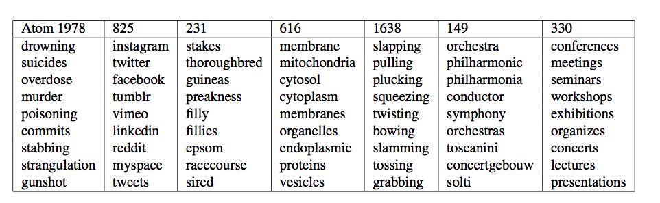
Each discourse atom defines via (2) a distribution on words, which due to the exponential appearing in (2) strongly favors words whose embeddings have a larger inner product with it. In practice, this distribution is quite concentrated on as few as 50-100 words, and the “meaning” of a discourse atom can be roughly determined by looking at a few nearby words. This is how we visualize atoms in the figures below. The first figure gives a few representative atoms of discourse.
And here are the discourse atoms used to represent two polysemous words, tie and spring
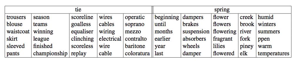
You can see that the discourse atoms do correspond to senses of these words.
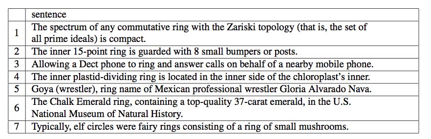
Finally, we also have a technique that, given a target word, generates representative sentences according to its various senses as detected by the algorithm. Below are the sentences returned for ring. (N.B. The mathematical meaning was missing in WordNet but was picked up by our method.)
A new testbed for testing comprehension of word senses
Many tests have been proposed to test an algorithm’s grasp of word senses. They often involve hard-to-understand metrics such as distance in WordNet, or sometimes tied to performance on specific applications like web search.
We propose a new simple test –inspired by word-intrusion tests for topic coherence due to Chang et al 2009– which has the advantages of being easy to understand, and can also be administered to humans.
We created a testbed using 200 polysemous words and their 704 senses according to WordNet. Each “sense” is represented by a set of 8 related words; these were collected from WordNet and online dictionaries by college students who were told to identify most relevant other words occurring in the online definitions of this word sense as well as in the accompanying illustrative sentences. These 8 words are considered as ground truth representation of the word sense: e.g., for the “tool/weapon” sense of axe they were: handle, harvest, cutting, split, tool, wood, battle, chop.
Police line-up test for word senses: the algorithm is given a random one of these 200 polysemous words and a set of $m$ senses which contain the true sense for the word as well as some distractors, which are randomly picked senses from other words in the testbed. The test taker has to identify the word’s true senses amont these $m$ senses.
As usual, accuracy is measured using precision (what fraction of the algorithm/human’s guesses were correct) and recall (how many correct senses were among the guesses).
For $m=20$ and $k=4$, our algorithm succeeds with precision $63\%$ and recall $70\%$, and performance remains reasonable for $m=50$. We also administered the test to a group of grad students. Native English speakers had precision/recall scores in the $75$ to $90$ percent range. Non-native speakers had scores roughly similar to our algorithm.
Our algorithm works something like this: If $w$ is the target word, then take all discourse atoms computed for that word, and compute a certain similarity score between each atom and each of the $m$ senses, where the words in the senses are represented by their word vectors. (Details are in the paper.)
Takeaways
Word embeddings have been useful in a host of other settings, and now it appears that they also can easily yield different senses of a polysemous word. We have some subsequent applications of these ideas to other previously studied settings, including topic models, creating WordNets for other languages, and understanding the semantic content of fMRI brain measurements. I’ll describe some of them in future posts.