From text translation to video captioning, learning to map one sequence to another is an increasingly active research area in machine learning. Fueled by the success of recurrent neural networks in its many variants, the field has seen rapid advances over the last few years. Recurrent neural networks are typically trained using some form of stochastic gradient descent combined with backpropagation for computing derivatives. The fact that gradient descent finds a useful set of parameters is by no means obvious. The training objective is typically non-convex. The fact that the model is allowed to maintain state is an additional obstacle that makes training of recurrent neural networks challenging.
In this post, we take a step back to reflect on the mathematics of recurrent neural networks. Interpreting recurrent neural networks as dynamical systems, we will show that stochastic gradient descent successfully learns the parameters of an unknown linear dynamical system even though the training objective is non-convex. Along the way, we’ll discuss several useful concepts from control theory, a field that has studied linear dynamical systems for decades. Investigating stochastic gradient descent for learning linear dynamical systems not only bears out interesting connections between machine learning and control theory, it might also provide a useful stepping stone for a deeper undestanding of recurrent neural networks more broadly.
Linear dynamical systems
We focus on time-invariant single-input single-output system. For an input sequence of real numbers $x_1,\dots, x_T\in \mathbb{R}$, the system maintains a sequence of hidden states $h_1,\dots, h_T\in \mathbb{R}^n$, and produces a sequence of outputs $y_1,\dots, y_T\in \mathbb{R}$ according to the following rules:
\[h_{t+1} = Ah_t + Bx_t~~~~~~~~~~~~~~~~~~~~~\] \[\quad \quad\quad~y_t = Ch_t+Dx_t+\xi_t ~~~~~~~~~~~~~~~~(1)\]Here $A,B,C,D$ are linear transformations with compatible dimensions, and $\xi_t$ is Gaussian noise added to the output at each time. In the learning problem, often called system identification in control theory, we observe samples of input-output pairs $((x_1,\dots, x_T),(y_1,\dots y_T))$ and aim to recover the parameters of the underlying linear system.
Although control theory provides a rich set of techniques for identifying and manipulating linear systems, maximum likelihood estimation with stochastic gradient descent remains a popular heuristic.
We denote by $\Theta = (A,B,C,D)$ the parameters of the true system. We parametrize our model with $\widehat{\Theta} = (\hat{A},\hat{B},\hat{C},\hat{D})$, and the trained model maintains hidden states $\hat{h}_t$ and outputs $\hat{y}_t$ exactly as in equation (1). For each given example $(x,y) = ((x_1,\dots,x_T), (y_1,\dots, y_t))$, the log-likelihood of model $\widehat{\Theta}$ is \(f(\widehat{\Theta}, (x,y)) = \frac{1}{T}\sum_{t=1}^{T}\left\|y_t-\hat{y}_t\right\|^2\). The population risk is defined as the expected log-likelihood,
\[f(\widehat{\Theta}) = \mathbb{E}_{(x,y)} \left[f(\widehat{\Theta}, (x,y))\right]\]Stochastic gradients of the population risk can be computed in time $O(Tn)$ via back-propagation given random samples. We can therefore directly minimize population risk using stochastic gradient descent. The question is just whether the algorithm actually converges. Even though the state transformations are linear, the objective function we defined is not convex. Luckily, we will see that the objective is still close enough to convex for stochastic gradient to make steady progress towards the global minimum.
Hair dryers and quasi-convex functions
Before we go into the math, let’s illustrate the algorithm with a pressing example that we all run into every morning: hair drying. Imagine you have a hair dryer with a low temperature setting and a high temperature setting. Neither setting is ideal. So every morning you switch between the settings frantically in an attempt to modulate to the ideal temperature. Measuring the resulting temperature (red line below) as a function of the input setting (green dots below), the picture you’ll see is something like this:

You can see that the output temperature is related to the inputs. If you set the temperature to high for long enough, you’ll eventually get a high output temperature. But the system has state. Briefly lowering the temperature has little effect on the outputs. Intuition suggests that these kind of effects should be captured by a system with two or three hidden states. So, let’s see how SGD would go about finding the parameters of the system. We’ll initialize a system with three hidden states such that before training its predictions are just the inputs of the system. We then run SGD with a fixed learning rate on the same sequence for 400 steps.

The blue line shows the predictions of SGD after 0/400 gradient updates. Click to advance.
Evidently, gradient descent converges just fine on this example. Let’s look at the hair dryer objective function along the line segment between two random points in the domain.

The function is clearly not convex, but it doesn’t look too bad either. In particular, from the picture, it could be that the objective function is quasi-convex:
Definition: For $\tau > 0$, a function $f(\theta)$ is $\tau$-quasi-convex with respect to a global minimum $\theta ^ * $ if for every $\theta$, \(\langle \nabla f(\theta), \theta - \theta^* \rangle \ge \tau (f(\theta)-f(\theta^*)).\)
Intuitively, quasi-convexity states that the descent direction $-\nabla f(\theta)$ is positively correlated with the ideal moving direction $\theta^* -\theta$. This implies that the potential function $\left|\theta-\theta ^ * \right|^2$ decreases in expectation at each step of stochastic gradient descent. This observation plugs nicely into the standard SGD analysis, leading to the following result:
Proposition: (informal) Suppose the population risk $f(\theta)$ is $\tau$-quasi-convex, then stochastic gradient descent (with fresh samples at each iteration and proper learning rate) converges to a point $\theta_K$ in $K$ iterations with error bounded by $ f(\theta_K) - f(\theta^*) \leq O(1/(\tau \sqrt{K}))$.
The key challenge for us is to understand under what conditions we can prove that the population risk objective is in fact quasi-convex. This requires some background.
Control theory, polynomial roots, and Pac-Man
A linear dynamical system $(A,B,C,D)$ is equivalent to the system $(TAT^{-1}, TB, CT^{-1}, D)$ for any invertible matrix $T$ in terms of the behavior of the outputs. A little thought shows therefore that in its unrestricted parameterization the objective function cannot have a unique optimum. A common way of removing this redundancy is to impose a canonical form. Almost all non-degenerate system admit the controllable canonical form, defined as
\[A\; = \; \left[ \begin{array}{ccccc} 0 & 1 & 0 & \cdots & 0 \newline 0 & 0 & 1 & \cdots & 0 \newline \vdots & \vdots & \vdots & \ddots & \vdots \newline 0 & 0 & 0 & \cdots & 1 \newline -a_n & -a_{n-1} & -a_{n-2} & \cdots & -a_1 \end{array} \right] \qquad B = \left[ \begin{array}{c} 0\newline 0 \newline\vdots \newline 0 \newline 1 \end{array} \right]\] \[C\;~= \; \left[ \begin{array}{ccccc} c_1~~~~& c_2~~~~ & c_3~~~~& ~~\cdots\cdots~~~~& c_n \end{array} \right] \qquad D =~~ \left[ \begin{array}{c} d\end{array} \right]\]We will also parametrize our training model using these forms. One of its nice properties is that the coefficients of the characteristic polynomial of the state transition matrix $A$ can be read off from the last row of $A$. That is, \(det(zI-A) = p_a(z) := z^n+a_1z^{n-1}+\dots + a_n.\)
Even in controllable canonical form, it still seems rather difficult to learn arbitrary linear dynamical systems. A natural restriction would be stability, that is, to require that the eigenvalues of $A$ are all bounded by $1.$ Equivalently, the roots of the characteristic polynomial should all be contained in the complex unit disc. Without stability, the state of the system could blow up exponentially making robust learning difficult. But the set of all stable systems forms a non-convex domain. It seems daunting to guarantee that stochastic gradient descent would converge from an arbtirary starting point in this domain without ever leaving the domain.
We will therefore impose a stronger restriction on the roots of the characteristic polynomial. We call this the Pac-Man condition. You can think of it as a strengthening of stability.
Pac-Man condition: A linear dynamical system in controllable canonical form satisfies the Pac-Man condition if the coefficient vector $a$ defining the state transition matrix satisfies \(|Re(q_a(z))| > |Im(q_a(z))|\) for all complex numbers $z$ of modulus $|z| = 1$, where $q_a(z) = p_a(z)/z^n = 1+a_1z^{-1}+\dots + a_nz^{-n}$.

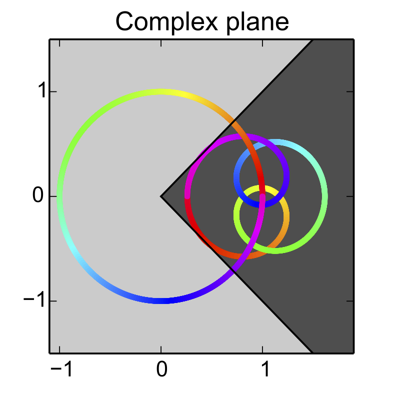
Above, we illustrate this condition for a degree 4 system plotting the value of $q_a(z)$ on complex plane for all complex numbers $z$ on the unit circle.
We note that Pac-Man condition is satisfied by vectors $a$ with $|a|_1\le \sqrt{2}/2$. Moreover, if $a$ is a random Gaussian vector with expected $\ell_2$ norm bounded by $o(1/\sqrt{\log n})$, then it will satisfy Pac-Man condition with probability $1-o(1)$. Roughly speaking, the assumption requires the roots of the characteristic polynomial $p_a(z)$ are relatively dispersed inside the unit circle.
The Pac-Man condition has three important implications:
-
It implies via Rouche’s theorem that the spectral radius of A is smaller than 1 and therefore ensures stability of the system.
-
The vectors satisfying it form a convex set in $\mathbb{R}^n$.
-
Finally, it ensures that the objective function is quasi-convex
Main result
Relying on the Pac-Man condition, we can show:
Main theorem (Hardt, Ma, Recht, 2016): Under the Pac-Man condition, projected gradient descent algorithm, given $N$ sample sequences of length $T$, returns parameters $\widehat{\Theta}$ with population risk \(f(\widehat{\Theta}) \le f(\Theta) + poly(n)/\sqrt{NT}.\)
The theorem sorts out the right dependence on $N$ and $T$. Even if there is only one sequence, we can learn the system provided that the sequence is long enough. Similarly, even if sequences are really short, we can learn provided that there are enough sequences.
Quasi-convexity in the frequency domain
To establish quasi-convexity under the Pac-Man condition, we will first develop an explicit formula for the population risk in frequency domain. In doing so, we assume that $x_1,\dots, x_T$ are pairwise independent with mean 0 and variance 1. We also consider the population risk as $T\rightarrow \infty$ for simplicity in this post.
A simple algebraic manipulation simplifies the population risk with infinite sequence length to
\[\lim_{T \rightarrow \infty} f(\widehat{\Theta}) = (\hat{D}-D)^2 + \sum_{k=0}^{\infty} (\hat{C}\hat{A}^kB-CA^k B)^2.\]The first term, $(\hat D - D)^2$ is convex and appears nowhere else. We can safely ignore it and focus on the remaining expression instead, which we call the idealized risk:
\[g(\widehat{\Theta}) = \sum_{k=0}^{\infty} (\hat{C}\hat{A}^kB-CA^k B)^2\]To deal with the sequence $\hat{C}\hat{A}^kB$, we take its Fourier transform and obtain that
\[\hat{C}\hat{A}^kB, k\ge 1 ~~~~\longrightarrow ~~~~~~~\widehat{G}_{\lambda} = \frac{\hat{c}_1e^{(n-1)\lambda}+\dots+ \hat{c}_n}{e^{n\lambda} + \hat{a}_1e^{(n-1)\lambda}+\dots+\hat{a}_n}, \lambda\in [0,2\pi]\]Similarly we take the Fourier transform of $CA^kB$, denoted by $G_{\lambda}$. Then by Parseval’s Theorem, we obtain the following alternative representation of the population risk,
\[f(\widehat{\Theta}) = \int_{0}^{2\pi} |G_{\lambda}-\widehat{G}_{\lambda}|^2 d\lambda.\]Mapping out $G_\lambda$ and $\widehat G_\lambda$ for all $\lambda\in [0, 2\pi]$ gives the following picture:
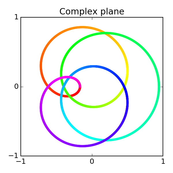
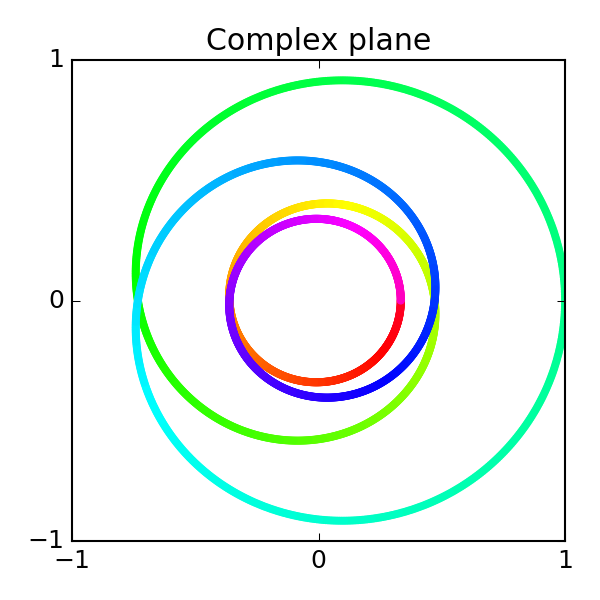
Left: Target transfer function $G$. Right: Approximation $\widehat G$ at step 0/10. Click to advance.
Given this pretty representation of the idealized risk objective, we can finally prove our main lemma.
Lemma: Suppose $\Theta$ satisfies the Pac-Man condition. Then, for every $0\le \lambda\le 2\pi$, $|G_{\lambda}-\widehat{G}_{\lambda}|^2$, as a function of $\hat{A},\hat{C}$ is quasi-convex in the Pac-Man region.
The lemma reduces to the following simple claim.
Claim: The function $h(\hat{u},\hat{v}) = |\hat{u}/\hat{v} - u/v|^2$ is quasi-convex in the region where $Re(\hat{v}/v) > 0$.
The proof simply involves computing the gradients and checking the conditions for quasi-convexity by elementary algebra. We omit a formal proof, but intead show a plot of the function $h(\hat{u}, \hat{v}) = (\hat{u}/\hat{v}- 1)^2$ over the reals:
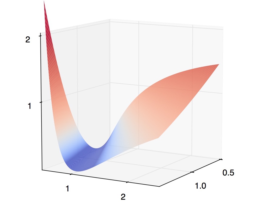
Click to rotate.
To see how the lemma follows from the previous claim we note that quasi-convexity is preserved under composition with any linear transformation. Specifically, $h(z)$ is quasi-convex, then $h(R x)$ is also quasi-convex for any linear map $R$. So, consider the linear map:
\[(\hat{a},\hat{c})\mapsto (\hat u, \hat v) = (\hat{c}_1e^{(n-1)\lambda}+\dots+ \hat{c}_n, e^{n\lambda} +\hat{a}_1e^{(n-1)\lambda}+\dots+\hat{a}_n)\]With this linear transformation, our simple claim about a bivariate function extends to show that $(G_{\lambda}-\widehat{G}_{\lambda})^2$ is quasi-convex when $Re(\hat{v}/v) \ge 0$. In particular, when $\hat{a}$ and $a$ both satisfy the Pac-Man condition, then $\hat{v}$ and $v$ both reside in the 90 degree wedge. Therefore they have an angle smaller than 90 degree. This implies that $Re(\hat{v}/v) > 0$.
Conclusion
We saw conditions under which stochastic gradient descent successfully learns a linear dynamical system. In our paper, we further show that allowing our learned system to have more parameters than the target system makes the problem dramatically easier. In particular, at the expense of slight over-parameterization we can weaken the Pac-Man condition to a mild separation condition on the roots of the characteristic polynomial. This is consistent with empirical observations both in machine learning and control theory that highlight the effectiveness of additional model parameters.
More broadly, we hope that our techniques will be a first stepping stone toward a better theoretical understanding of recurrent neural networks.