Given the sheer number of backpropagation tutorials on the internet, is there really need for another? One of us (Sanjeev) recently taught backpropagation in undergrad AI and couldn’t find any account he was happy with. So here’s our exposition, together with some history and context, as well as a few advanced notions at the end. This article assumes the reader knows the definitions of gradients and neural networks.
What is backpropagation?
It is the basic algorithm in training neural nets, apparently independently rediscovered several times in the 1970-80’s (e.g., see Werbos’ Ph.D. thesis and book, and Rumelhart et al.). Some related ideas existed in control theory in the 1960s. (One reader points out another independent rediscovery, the Baur-Strassen lemma from 1983.)
Backpropagation gives a fast way to compute the sensitivity of the output of a neural network to all of its parameters while keeping the inputs of the network fixed: specifically it computes all partial derivatives ${\partial f}/{\partial w_i}$ where $f$ is the output and $w_i$ is the $i$th parameter. (Here parameters can be edge weights or biases associated with nodes or edges of the network, and the precise details of the node computations —e.g., the precise form of nonlinearity like Sigmoid or RELU— are unimportant.) Doing so gives the gradient $\nabla f$ of $f$ with respect to its network parameters, which allows a gradient descent step in the training: change all parameters simultaneously to move the vector of parameters a small amount in the direction $-\nabla f$.
Note that backpropagation computes the gradient exactly, but properly training neural nets needs many more tricks than just backpropagation. Understanding backpropagation is useful for appreciating some advanced tricks.
The importance of backpropagation derives from its efficiency. Assuming node operations take unit time, the running time is linear, specifically, $O(\text{Network Size}) = O(V + E)$, where $V$ is the number of nodes in the network and $E$ is the number of edges. The only technical ingredient is chain rule from calculus, but applying it naively would have resulted in quadratic running time—which would be hugely inefficient for networks with millions or even thousands of parameters.
Backpropagation can be efficiently implemented using highly parallel vector operations available in today’s GPUs (Graphical Processing Units), which play an important role in the the recent neural nets revolution.
Side Note: Expert readers will recognize that in the standard accounts of neural net training, the actual quantity of interest is the gradient of the training loss, which happens to be a simple function of the network output. But the above phrasing is fully general since one can simply add a new output node to the network that computes the training loss from the old output. Then the quantity of interest is indeed the gradient of this new output with respect to network parameters.
Problem Setup
Backpropagation applies only to acyclic networks with directed edges. (Later we briefly sketch its use on networks with cycles.)
Without loss of generality, acyclic networks can be visualized as being structured in numbered layers, with nodes in the $t+1$th layer getting all their inputs from the outputs of nodes in layers $t$ and earlier. We use $f \in \mathbb{R}$ to denote the output of the network. In all our figures, the input of the network is at the bottom and the output on the top.
We start with a simple claim that reduces the problem of computing the gradient to the problem of computing partial derivatives with respect to the nodes:
Claim 1: To compute the desired gradient with respect to the parameters, it suffices to compute $\partial f/\partial u$ for every node $u$.
Let’s be clear what $\partial f/\partial u$ means. Suppose we cut off all the incoming edges of the node $u$, and fix/clamp the current values of all network parameters. Now imagine changing $u$ from its current value. This change may affect values of nodes at higher levels that are connected to $u$, and the final output $f$ is one such node. Then $\partial f/\partial u$ denotes the rate at which $f$ will change as we vary $u$. (Aside: Readers familiar with the usual exposition of back-propagation should note that there $f$ is the training error and this $\partial f/\partial u$ turns out to be exactly the “error” propagated back to on the node $u$.)
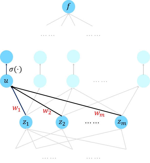
Claim 1 is a direct application of chain rule, and let’s illustrate it for a simple neural nets (we address more general networks later). Suppose node $u$ is a weighted sum of the nodes $z_1,\dots, z_m$ (which will be passed through a non-linear activation $\sigma$ afterwards). That is, we have $u = w_1z_1+\dots+w_nz_n$. By Chain rule, we have
\[\frac{\partial f}{\partial w_1} = \frac{\partial f}{\partial u}\cdot \frac{\partial{u}}{\partial w_1} = \frac{\partial f}{\partial u}\cdot z_1.\]Hence, we see that having computed $\partial f/\partial u$ we can compute $\partial f/\partial w_1$, and moreover this can be done locally by the endpoints of the edge where $w_1$ resides.

Multivariate Chain Rule
Towards computing the derivatives with respect to the nodes, we first recall the multivariate Chain rule, which handily describes the relationships between these partial derivatives (depending on the graph structure).
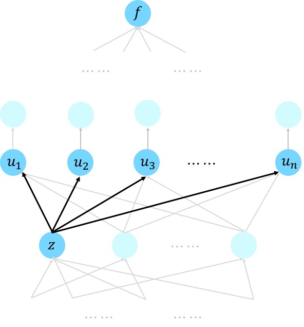
Suppose a variable $f$ is a function of variables $u_1,\dots, u_n$, which in turn depend on the variable $z$. Then, multivariate Chain rule says that
\[\frac{\partial f}{\partial z} = \sum_{j=1}^n \frac{\partial f}{\partial u_j}\cdot \frac{\partial u_j}{\partial z}~.\]This is a direct generalization of eqn. (2) and a sub-case of eqn. (11) in this description of chain rule.
This formula is perfectly suitable for our cases. Below is the same example as we used before but with a different focus and numbering of the nodes.

We see that given we’ve computed the derivatives with respect to all the nodes that is above the node $z$, we can compute the derivative with respect to the node $z$ via a weighted sum, where the weights involve the local derivative ${\partial u_j}/{\partial z}$ that is often easy to compute. This brings us to the question of how we measure running time. For book-keeping, we assume that
Basic assumption: If $u$ is a node at level $t+1$ and $z$ is any node at level $\leq t$ whose output is an input to $u$, then computing $\frac{\partial u}{\partial z}$ takes unit time on our computer.
Naive feedforward algorithm (not efficient!)
It is useful to first point out the naive quadratic time algorithm implied by the chain rule. Most authors skip this trivial version, which we think is analogous to teaching sorting using only quicksort, and skipping over the less efficient bubblesort.
The naive algorithm is to compute $\partial u_i/\partial u_j$ for every pair of nodes where $u_i$ is at a higher level than $u_j$. Of course, among these $V^2$ values (where $V$ is the number of nodes) are also the desired ${\partial f}/{\partial u_i}$ for all $i$ since $f$ is itself the value of the output node.
This computation can be done in feedforward fashion. If such value has been obtained for every $u_j$ on the level up to and including level $t$, then one can express (by inspecting the multivariate chain rule) the value $\partial u_{\ell}/\partial u_j$ for some $u_{\ell}$ at level $t+1$ as a weighted combination of values $\partial u_{i}/\partial u_j$ for each $u_i$ that is a direct input to $u_{\ell}$. This description shows that the amount of computation for a fixed $j$ is proportional to the number of edges $E$. This amount of work happens for all $V$ values of $j$, letting us conclude that the total work in the algorithm is $O(VE)$.
Backpropagation (Linear Time)
The more efficient backpropagation, as the name suggests, computes the partial derivatives in the reverse direction. Messages are passed in one wave backwards from higher number layers to lower number layers. (Some presentations of the algorithm describe it as dynamic programming.)
Messaging protocol: The node $u$ receives a message along each outgoing edge from the node at the other end of that edge. It sums these messages to get a number $S$ (if $u$ is the output of the entire net, then define $S=1$) and then it sends the following message to any node $z$ adjacent to it at a lower level: \(S \cdot \frac{\partial u}{\partial z}\)
Clearly, the amount of work done by each node is proportional to its degree, and thus overall work is the sum of the node degrees. Summing all node degrees counts each edge twice, and thus the overall work is $O(\text{Network Size})$.
To prove correctness, we prove the following:
Main Claim: At each node $z$, the value $S$ is exactly ${\partial f}/{\partial z}$.
Base Case: At the output layer this is true, since ${\partial f}/{\partial f} =1$.
Inductive case: Suppose the claim was true for layers $t+1$ and higher and $u$ is at layer $t$, with outgoing edges go to some nodes $u_1, u_2, \ldots, u_m$ at levels $t+1$ or higher. By inductive hypothesis, node $z$ indeed receives $ \frac{\partial f}{\partial u_j}\times \frac{\partial u_j}{\partial z}$ from each of $u_j$. Thus by Chain rule, \(S= \sum_{i =1}^m \frac{\partial f}{\partial u_i}\frac{\partial u_i}{\partial z}=\frac{\partial f}{\partial z}.\) This completes the induction and proves the Main Claim.
Auto-differentiation
Since the exposition above used almost no details about the network and the operations that the node perform, it extends to every computation that can be organized as an acyclic graph whose each node computes a differentiable function of its incoming neighbors. This observation underlies many auto-differentiation packages such as autograd or tensorflow: they allow computing the gradient of the output of such a computation with respect to the network parameters.
We first observe that Claim 1 continues to hold in this very general setting. This is without loss of generality because we can view the parameters associated to the edges as also sitting on the nodes (actually, leaf nodes). This can be done via a simple transformation to the network; for a single node it is shown in the picture below; and one would need to continue to do this transformation in the rest of the networks feeding into $u_1, u_2,..$ etc from below.
Then, we can use the messaging protocol to compute the derivatives with respect to the nodes, as long as the local partial derivative can be computed efficiently. We note that the algorithm can be implemented in a fairly modular manner: For every node $u$, it suffices to specify (a) how it depends on the incoming nodes, say, $z_1,\dots, z_n$ and (b) how to compute the partial derivative times $S$, that is, $S \cdot \frac{\partial u}{\partial z_j}$.
Extension to vector messages: In fact (b) can be done efficiently in more general settings where we allow the output of each node in the network to be a vector (or even matrix/tensor) instead of only a real number. Here we need to replace $\frac{\partial u}{\partial z_j}\cdot S$ by $\frac{\partial u}{\partial z_j}[S]$, which denotes the result of applying the operator $\frac{\partial u}{\partial z_j}$ on $S$. We note that to be consistent with the convention in the usual exposition of backpropagation, when $y\in \mathbb{R}^{p}$ is a funciton of $x\in \mathbb{R}^q$, we use $\frac{\partial y}{\partial x}$ to denote $q\times p$ dimensional matrix with $\partial y_j/\partial x_i$ as the $(i,j)$-th entry. Readers might notice that this is the transpose of the usual Jacobian matrix defined in mathematics. Thus $\frac{\partial y}{\partial x}$ is an operator that maps $\mathbb{R}^p$ to $\mathbb{R}^q$ and we can verify $S$ has the same dimension as $u$ and $\frac{\partial u}{\partial z_j}[S]$ has the same dimension as $z_j$.
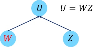
For example, as illustrated below, suppose the node $U\in \mathbb{R}^{d_1\times d_3} $ is a product of two matrices $W\in \mathbb{R}^{d_2\times d_3}$ and $Z\in \mathbb{R}^{d_1\times d_2}$. Then we have that $\partial U/\partial Z$ is a linear operator that maps $\mathbb{R}^{d_2\times d_3}$ to $\mathbb{R}^{d_1\times d_3}$, which naively requires a matrix representation of dimension $d_2d_3\times d_1d_3$. However, the computation (b) can be done efficiently because \(\frac{\partial U}{\partial Z}[S]= W^{\top}S.\)
Such vector operations can also be implemented efficiently using today’s GPUs.

Notable Extensions
1) Allowing weight tying. In many neural architectures, the designer wants to force many network units such as edges or nodes to share the same parameter. For example, in convolutional neural nets, the same filter has to be applied all over the image, which implies reusing the same parameter for a large set of edges between the two layers.
For simplicity, suppose two parameters $a$ and $b$ are supposed to share the same value. This is equivalent to adding a new node $u$ and connecting $u$ to both $a$ and $b$ with the operation $a = u$ and $b=u$. Thus, by chain rule, \(\frac{\partial f}{\partial u} = \frac{\partial f}{\partial a}\cdot \frac{\partial a}{\partial u}+\frac{\partial f}{\partial b}\cdot \frac{\partial b}{\partial u} = \frac{\partial f}{\partial a}+ \frac{\partial f}{\partial b}.\) Hence, equivalently, the gradient with respect to a shared parameter is the sum of the gradients with respect to individual occurrences.
2) Backpropagation on networks with loops. The above exposition assumed the network is acyclic. Many cutting-edge applications such as machine translation and language understanding use networks with directed loops (e.g., recurrent neural networks). These architectures —all examples of the “differentiable computing” paradigm below—can get complicated and may involve operations on a separate memory as well as mechanisms to shift attention to different parts of data and memory.
Networks with loops are trained using gradient descent as well, using back-propagation through time, which consists of expanding the network through a finite number of time steps into an acyclic graph, with replicated copies of the same network. These replicas share the weights (weight tying!) so the gradient can be computed. In practice an issue may arise with exploding or vanishing gradients which impact convergence. Such issues can be carefully addressed in practice by clipping the gradient or re-parameterization techniques such as long short-term memory.
The fact that the gradient can be computed efficiently for such general networks with loops has motivated neural net models with memory or even data structures (see for example neural Turing machines and differentiable neural computer). Using gradient descent, one can optimize over a family of parameterized networks with loops to find the best one that solves a certain computational task (on the training examples). The limits of these ideas are still being explored.
3) Hessian-vector product in linear time. It is possible to generalize backprop to enable 2nd order optimization in “near-linear” time, not just gradient descent, as shown in recent independent manuscripts of Carmon et al. and Agarwal et al. (NB: Tengyu is a coauthor on this one.). One essential step is to compute the product of the Hessian matrix and a vector, for which Pearlmutter’93 gave an efficient algorithm. Here we show how to do this in $O(\mbox{Network size})$ using the ideas above. We need a slightly stronger version of the back-propagation result than the one in the previous subsection:
Claim (informal): Suppose an acyclic network with $V$ nodes and $E$ edges has output $f$ and leaves $z_1,\dots, z_m$. Then there exists a network of size $O(V+E)$ that has $z_1,\dots, z_m$ as input nodes and $\frac{\partial f}{\partial z_1},\dots, \frac{\partial f}{\partial z_m}$ as output nodes.
The proof of the Claim follows in straightforward fashion from implementing the message passing protocol as an acyclic circuit.
Next we show how to compute $\nabla^2 f(z)\cdot v$ where $v$ is a given fixed vector. Let $g(z)= \langle \nabla f(z),v\rangle$ be a function from $\mathbb{R}^d\rightarrow \mathbb{R}$. Then by the Claim above, $g(z)$ can be computed by a network of size $O(V+E)$. Now apply the Claim again on $g(z)$, we obtain that $\nabla g(z)$ can also be computed by a network of size $O(V+E)$.
Note that by construction, \(\nabla g(z) = \nabla^2 f(z)\cdot v.\) Hence we have computed the Hessian vector product in network size time.
##That’s all!
Please write your comments on this exposition and whether it can be improved.
