This is yet another post about Generative Adversarial Nets (GANs), and based upon our new ICLR’18 paper with Yi Zhang. A quick recap of the story so far. GANs are an unsupervised method in deep learning to learn interesting distributions (e.g., images of human faces), and also have a plethora of uses for image-to-image mappings in computer vision. Standard GANs training is motivated using this task of distribution learning, and is designed with the idea that given large enough deep nets and enough training examples, as well as accurate optimization, GANs will learn the full distribution.
Sanjeev’s previous post concerned his co-authored ICML’17 paper which called this intuition into question when the deep nets have finite capacity. It shows that the training objective has near-equilibria where the discriminator is fooled —i.e., training objective is good—but the generator’s distributions has very small support, i.e. shows mode collapse. This is a failure of the model, and raises the question whether such bad equilibria are found in real-life training. A second post showed empirical evidence that they do, using the birthday-paradox test.
The current post concerns our new result (part of our upcoming ICLR paper) which shows that bad equilibria exist also in more recent GAN architectures based on simultaneously learning an encoder and decoder. This should be surprising because many researchers believe that encoder-decoder architectures fix many issues with GANs, including mode collapse.
As we will see, encoder-decoder GANs seem very powerful. In particular, the proof of the previously mentioned negative result utterly breaks down for this architecture. But, we then discovered a cute argument that shows encoder-decoder GANs can have poor solutions, featuring not only mode collapse but also encoders that map images to nonsense (more precisely Gaussian noise). This is the worst possible failure of the model one could imagine.
Encoder-decoder architectures
Encoders and decoders have long been around in machine learning in various forms – especially deep learning. Speaking loosely, underlying all of them are two basic assumptions:
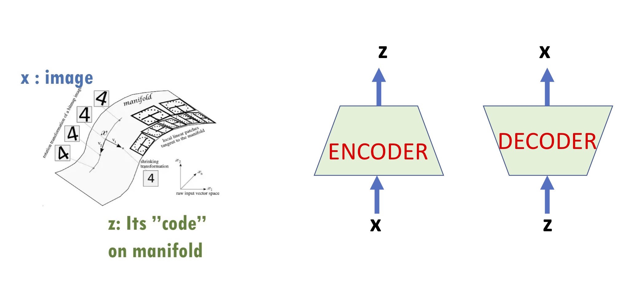
(1) Some form of the so-called manifold assumption which asserts that high-dimensional data such as real-life images lie (roughly) on a low-dimensional manifold. (“Manifold” should be interpreted rather informally – sometimes this intuition applies only very approximately sometimes it’s meant in a “distributional” sense, etc.)
(2) The low-dimensional structure is “meaningful”: if we think of an image $x$ as a high-dimensional vector and its “code” $z$ as its coordinates on the low-dimensional manifold, the code $z$ is thought of as a “high-level” descriptor of the image.
With the above two points in mind, an encoder maps the image to its code, and a decoder computes the reverse map. (We also discussed encoders and decoders in our earlier post on representation learning in a more general setup.)
Encoder-Decoder GANs
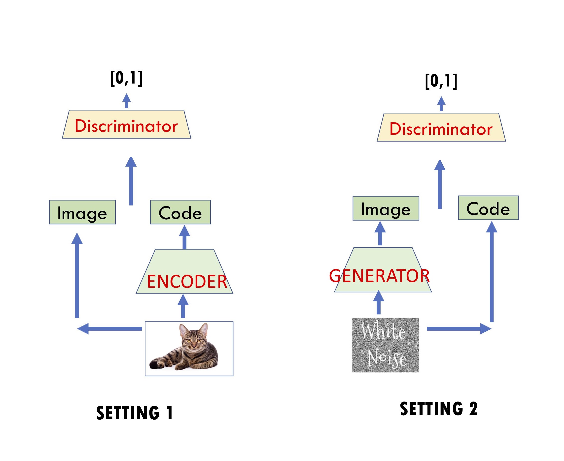
These were introduced by Dumoulin et al.(ALI) and Donahue et al.(BiGAN). They involve two competitors: Player 1 involves a discriminator net $D$ that is given an input of the form (image, code) and it outputs a number in the interval $[0,1]$, which denotes its “satisfaction level” with this input. Player 2 trains a decoder net $G$ (also called generator in the GANs setting) and an encoder net $E$.
Recall that in the standard GAN, discriminator tries to distinguish real images from images generated by the generator $G$. Here discriminator’s input is an image and its code. Specifically, Player 1 is trying to train its net to distinguish between the following two settings, and Player 2 is trying to make sure the two settings look indistinguishable to Player 1’s net.
\(\mbox{Setting 1: presented with}~(x, E(x))~\mbox{where $x$ is random real image}.\) \(\mbox{Setting 2: presented with}~(G(z), z)~\mbox{where $z$ is random code}.\)
(Here it is assumed that a random code is a vector with i.i.d gaussian coordinates, though one could consider other distributions.)
The hoped-for equilibrium obviously is one where generator and encoder are inverses of each other: $E(G(z)) \approx z$ and $G(E(x)) \approx x$, and the joint distributions $(z,G(z))$ and $(E(x), x)$ roughly match. The underlying intuition is that if this happens, Player 1 must’ve produced a “meaningful” representation $E(x)$ for the images – and this should improve the quality of the generator as well. Indeed, Dumoulin et al.(ALI) provide some small-scale empirical examples on mixtures of Gaussians for which encoder-decoder architectures seem to ameliorate the problem of mode collapse.
The above papers prove that when the encoder/decoder/discriminator have infinite capacity, the desired solution is indeed an equilibrium. However, we’ll see that things are very different when capacities are finite.
Finite-capacity discriminators are weak
Say a generator/encoder pair $(G,E)$ $\epsilon$-fools a decoder $D$ if
\[|E_{x} D(x, E(x)) - E_{z} D(G(z), z)| \leq \epsilon\]In other words, $D$ has roughly similar output in Settings 1 and 2.
Our theorem applies when the distribution consists of realistic images, as explained later. We show the following:
(Informal theorem) If the discriminator $D$ has capacity (i.e. number of parameters) at most $p$, then there is an encoder $E$ of capacity $\ll p$ and generator $G$ of slightly larger capacity than $p$ such that $(G, E)$ can $\epsilon$-fool every such $D$. Furthermore, the generator exhibits mode collapse: its distribution is essentially supported on a bit more than $p$ images, and the encoder $E$ just outputs white noise (i.e. does not extract any “meaningful” representation) given an image.
(Note that such a $(G, E)$ represents an $\epsilon$-approximate equilibrium, in the sense that player 1 cannot gain more than $\epsilon$ in the distinguishing probability by switching its discriminator. )
It is important that the encoder’s capacity is much less than $p$, and thus the theorem allows a discriminator that is able to simulate $E$ if it needed, and in particular verify for a random seed $z$ that $E(G(z)) \approx z$. The theorem says that even the ability to conduct such a verification cannot give it power to force encoder to produce meaningful codes. This is a counterintuitive aspect of the result. The main difficulty in the proof (which stumped us for a bit) was how to exhibit such an equilibrium where $E$ is a small net.
This is ensured by a simple assumption. We assume the image distribution is mildly “noised”: say, every 100th pixel is replaced by Gaussian noise. To a human, such an image would of course be indistinguishable from a real image. (NB: Our proof could be carried out via some other assumptions to the effect that images have an innate stochastic/noise component that is efficiently extractable by a small neural network. But let’s keep things clean.) When noise $\eta$ is thus added to an image $x$, we denote the resulting image as $x \odot \eta$.
Now the encoder will be rather trivial: given the noised image $x \odot \eta$, output $\eta$. Clearly, such an encoder does not in any sense capture “meaning” in the image. It is also implementable by a tiny single-layer net, as required by the theorem.
Construction of generator
As usual in the GAN literature, we will assume the discriminator is $L$-Lipschitz. This can be a loose upperbound, since only $\log L$ enters quantitatively in the proof.
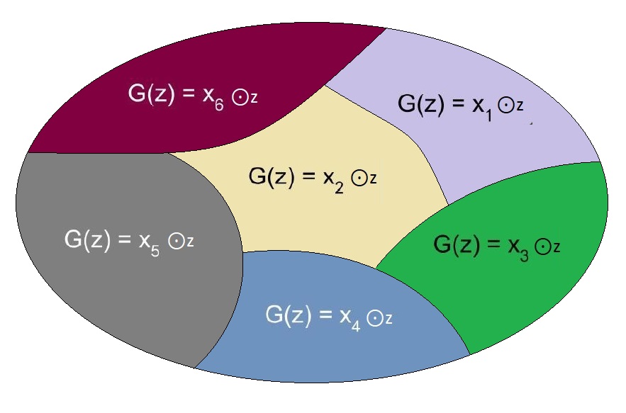
The generator $G(z)$ in the theorem statement memorizes a hash function that partitions the set of all seeds/codes $z$ into $m$ equal-sized blocks; it also memorizes a “pool” of $m := p \log^2(pL)/ \epsilon^2$ unnoised images $\tilde{x}_1, \tilde{x}_2, \dots, \tilde{x}_m$. When presented with a random seed $z$, the generator computes the block of the partition that $z$ lies in, and then produces the image $\tilde{x}_i \odot z$, where $i$ is the block $z$ belongs to. (See the Figure below.)
Now we have to prove that such a memorizing generator exists that $\epsilon$-fools all discriminators of capacity $p$. This is shown by the probabilistic method: we describe a distribution over generators $G$ that works “in expectation”, and subsequently use concentration bounds to prove there exists at least one generator that does the job.
The distribution on $G$’s is straightforward: we select the pool of (unnoised) images $\tilde{x}_1, \tilde{x}_2, .., \tilde{x}_m$ at random. Why is this distribution for $G$ sensible? Notice the following simple fact:
\[E_{G} E_{z} D(G(z), z) = E_{\tilde{x}, z} D(\tilde{x} \odot z, z) = E_{x} D(x, E(x)) \hspace{2cm} (3)\]In other words, the “expected” encoder correctly matches the expectation of $D(x, E(x))$, so that the discriminator is fooled “in expectation”. This of course is not enough: we need some kind of concentration argument to show a particular $G$ works against all possible discriminators, which will ultimately use the fact that the discriminator $D$ has a small capacity and small Lipschitz constant. (Think covering number arguments in learning theory.)
Towards that, another useful observation: if $q$ is the uniform distribution over sets $T= {z_1, z_2,\dots, z_m}$, s.t. each $z_i$ is independently sampled from the conditional distribution inside the $i$-th block of the partition of the noise space, by the law of total expectation one can see that \(E_{z} D(G(z), z) = E_{T \sim q} \frac{1}{m} \sum_{i=1}^m D(G(z_i), z_i)\) The right hand side is an average of terms, each of which is a bounded function of mutually independent random variables – so, by e.g. McDiarmid’s inequality it concentrates around it’s expectation, which by (3) is exactly $E_{z} D(G(z), z)$.
To finish the argument off, we use the fact that due to Lipschitzness and the bound on the number of parameters, the “effective” number of distinct discriminators is small, so we can union bound over them. (Formally, this translates to an epsilon-net + union bound argument. This also gives rise to the value of $m$ used in the construction.)
Takeaway
The result should be interpreted as saying that possibly the theoretical foundations of GANs need more work. The current way of thinking about them as distribution learners may not be the right way to formalize them. Furthermore, one has to take care about transfering notions invented for distribution learning, such as encoders and decoders, over into the GANs setting. Finally there is an empirical question whether any of the myriad GANS variations can avoid mode collapse.