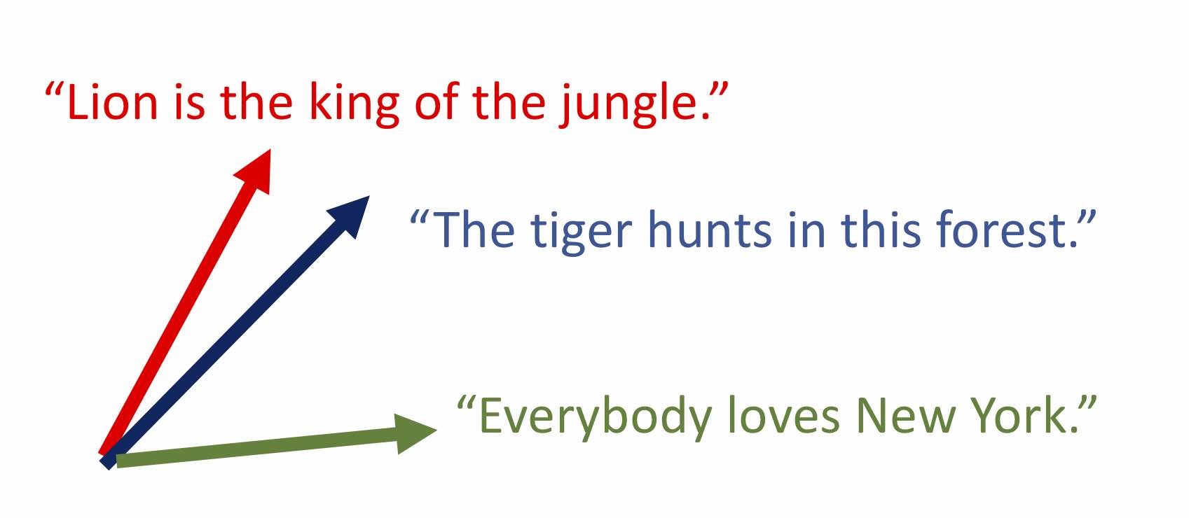
Word embeddings (see my old post1 and post2) capture the idea that one can express “meaning” of words using a vector, so that the cosine of the angle between the vectors captures semantic similarity. (“Cosine similarity” property.) Sentence embeddings and text embeddings try to achieve something similar: use a fixed-dimensional vector to represent a small piece of text, say a sentence or a small paragraph. The performance of such embeddings can be tested via the Sentence Textual Similarity (STS) datasets (see the wiki page), which contain sentence pairs humanly-labeled with similarity ratings.
A general hope behind computing text embeddings is that they can be learnt using a large unlabeled text corpus (similar to word embeddings) and then allow good performance on downstream classification tasks with few labeled examples. Thus the overall pipeline could look like this:
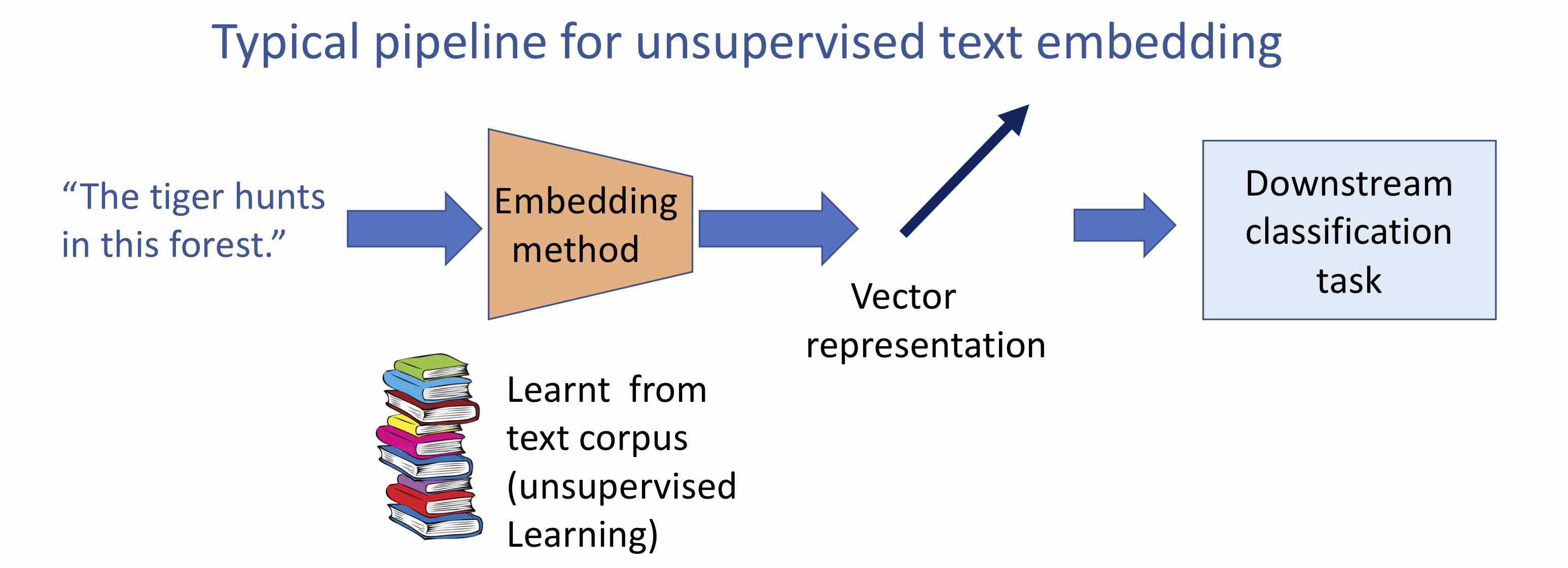
Computing such representations is a form of representation learning as well as unsupervised learning. This post will be an introduction to extremely simple ways of computing sentence embeddings, which on many standard tasks, beat many state-of-the-art deep learning methods. This post is based upon my ICLR’17 paper on SIF embeddings with Yingyu Liang and Tengyu Ma.
Existing methods
Topic modeling is a classic technique for unsupervised learning on text and it also yields a vector representation for a paragraph (or longer document), specifically, the vector of “topics” occuring in this document and their relative proportions. Unfortunately, topic modeling is not accurate at producing good representations at the sentence or short paragraph level, and furthermore there appears to be no variant of topic modeling that leads to the good cosine similarity property that we desire.
Recurrent neural net is the default deep learning technique to train a language model. It scans the text from left to right, maintaining a fixed-dimensional vector-representation of the text it has seen so far. It’s goal is to use this representation to predict the next word at each time step, and the training objective is to maximise log-likelihood of the data (or similar). Thus for example, a well-trained model when given a text fragment “I went to the cafe and ordered a ….” would assign high probability to “coffee”, “croissant” etc. and low probability to “puppy”. Myriad variations of such language models exist, many using biLSTMs which have some long-term memory and can scan the text forward and backwards. Lately biLSTMs have been replaced by convolutional architectures with attention mechanism; see for instance this paper.
One obtains a text representation by peeking at the internal representation (i.e., node activations) at the top layer of this deep model. After all, when the model is scanning through text, its ability to predict the next word must imply that this internal representation implicitly captures a gist of all it has seen, reflecting rules of grammar, common-sense etc. (e.g., that you don’t order a puppy at a cafe). Some notable modern efforts along such lines are Hierarchichal Neural Autoencoder of Li et al. as well as Palangi et al, and Skipthought of Kiros et al..
As with all deep learning models, one wishes for interpretability: what information exactly did the machine choose to put into the text embedding? Besides the usual reasons for seeking interpretability, in an NLP context it may help us leverage additional external resources such as WordNet in the task. Other motivations include transfer learning/domain adaptation (to solve classification tasks for a small text corpus, leverage text embeddings trained on a large unrelated corpus).
Surprising power of simple linear representations
In practice, many NLP applications rely on a simple sentence embedding: the average of the embeddings of the words in it. This makes some intuitive sense, because recall that the Word2Vec paper uses the following expression (in the their simpler CBOW word embedding)
\[\Pr[w~|~w_1,w_2, w_3, w_4, w_5] \propto \exp(v_w \cdot (\frac{1}{5} \sum_i v_{w_i}). \qquad (1)\]which suggests that the sense of a sequence of words is captured via simple average of word vectors.
While this simple average has only fair performance in capturing sentence similarity via cosine similarity, it can be quite powerful in downstream classification tasks (after passing through a single layer neural net) as shown in a surprising paper of Wieting et al. ICLR’16.
Better linear representation: SIF embeddings
My ICLR’17 paper with Yingyu Liang and Tengyu Ma improved such simple averaging using our SIF embeddings. They’re motivated by the empirical observation that word embeddings have various pecularities stemming from the training method, which tries to capture word cooccurence probabilities using vector inner product, and words sometimes occur out of context in documents. These anomalies cause the average of word vectors to have nontrivial components along semantically meaningless directions. SIF embeddings try to combat this in two ways, which I describe intuitively first, followed by more theoretical justification.
Idea 1: Nonuniform weighting of words. Conventional wisdom in information retrieval holds that “frequent words carry less signal.” Usually this is captured via TF-IDF weighting, which assigns weightings to words inversely proportional to their frequency. We introduce a new variant we call Smoothed Inverse Frequency (SIF) weighting, which assigns to word $w$ a weighting $\alpha_w = a/(a+ p_w)$ where $p_w$ is the frequency of $w$ in the corpus and $a$ is a hyperparameter. Thus the embedding of a piece of text is $\sum_w \alpha_w v_w$ where the sum is over words in it. (Aside: word frequencies can be estimated from any sufficiently large corpus; we find embedding quality to be not too dependent upon this.)
On a related note, we found that folklore understanding of word2vec, viz., expression (1), is false. A dig into the code reveals a resampling trick that is tantamount to a weighted average quite similar to our SIF weighting. (See Section 3.1 in our paper for a discussion.)
Idea 2: Remove component from top singular direction. The next idea is to modify the above weighted average by removing the component in a special direction, corresponding to the top singular direction set of weighted embeddings of a smallish sample of sentences from the domain (if doing domain adaptation, component is computed using sentences of the target domain). The paper notes that the direction corresponding to the top singular vector tends to contain information related to grammar and stop words, and removing the component in this subspace really cleans up the text embedding’s ability to express meaning.
Theoretical justification
A notable part of our paper is to give a theoretical justification for this weighting using a generative model for text similar to one used in our word embedding paper in TACL’16 as described in my old post. That model tries to give the causative relationship between word meanings and their cooccurence probabilities. It thinks of corpus generation as a dynamic process, where the $t$-th word is produced at step $t$. The model says that the process is driven by the random walk of a discourse vector $c_t \in \Re^d$. It is a unit vector whose direction in space represents what is being talked about. Each word has a (time-invariant) latent vector $v_w \in \Re^d$ that captures its correlations with the discourse vector. We model this bias with a loglinear word production model:
\[\Pr[w~\mbox{emitted at time $t$}~|~c_t] \propto \exp(c_t\cdot v_w). \qquad (2)\]The discourse vector does a slow geometric random walk over the unit sphere in $\Re^d$. Thus $c_{t+1}$ is obtained by a small random displacement from $c_t$. Since expression (2) places much higher probability on words that are clustered around $c_t$, and $c_t$ moves slowly. If the discourse vector moves slowly, then we can assume a single discourse vector gave rise to the entire sentence or short paragraph. Thus given a sentence, a plausible vector representation of its “meaning” is a max a posteriori (MAP) estimate of the discourse vector that generated it.
Such models have been empirically studied for a while, but our paper gave a theoretical analysis, and showed that various subcases imply standard word embedding methods such as word2vec and GloVe. For example, it shows that MAP estimate of the discourse vector is the simple average of the embeddings of the preceding $k$ words – in other words, the average word vector!
This model is clearly simplistic and our ICLR’17 paper suggests two correction terms, intended to account for words occuring out of context, and to allow some common words (“the”, “and”, “but” etc.) appear often regardless of the discourse. We first introduce an additive term $\alpha p(w)$ in the log-linear model, where $p(w)$ is the unigram probability (in the entire corpus) of word and $\alpha$ is a scalar. This allows words to occur even if their vectors have very low inner products with $c_s$. Secondly, we introduce a common discourse vector $c_0\in \Re^d$ which serves as a correction term for the most frequent discourse that is often related to syntax. It boosts the co-occurrence probability of words that have a high component along $c_0$.(One could make other correction terms, which are left to future work.) To put it another way, words that need to appear a lot out of context can do so by having a component along $c_0$, and the size of this component controls its probability of appearance out of context.
Concretely, given the discourse vector $c_s$ that produces sentence $s$, the probability of a word $w$ is emitted in the sentence $s$ is modeled as follows, where $\tilde{c}_{s} = \beta c_0 + (1-\beta) c_s, c_0 \perp c_s$, $\alpha$ and $\beta$ are scalar hyperparameters:
\[\Pr[w \mid s] = \alpha p(w) + (1-\alpha) \frac{\exp(<\tilde{c}_{s}, v_w>)}{Z_{\tilde{c,s}}},\]where
\[Z_{\tilde{c,s}} = \sum_{w} \exp(<\tilde{c}_{s}, v_w>)\]is the normalizing constant (the partition function). We see that the model allows a word $w$ unrelated to the discourse $c_s$ to be emitted for two reasons: a) by chance from the term $\alpha p(w)$; b) if $w$ is correlated with the common direction $c_0$.
The paper shows that the MAP estimate of the $c_s$ vector corresponds to the SIF embeddings described earlier, where the top singular vector used in their construction is an estimate of the $c_0$ vector in the model.
Empirical performance
The performance of this embedding scheme appears in the figure below. Note that Wieting et al. had already shown that their method (which is semi-supervised, relying upon a large unannotated corpus and a small annotated corpus) beats many LSTM-based methods. So this table only compares to their work; see the papers for comparison with more past work.
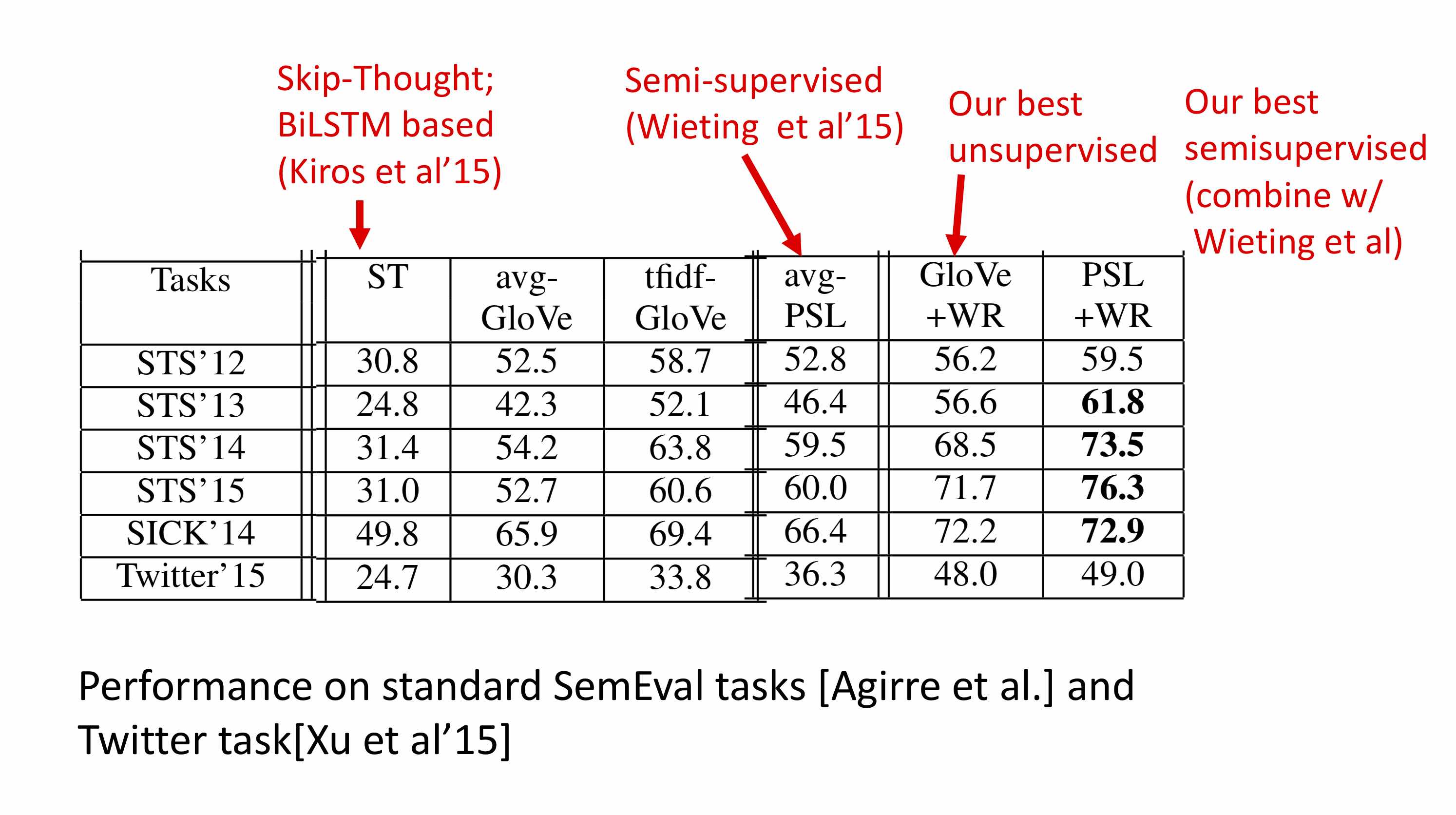
For other performance results please see the paper.
Next post
In the next post, I will sketch improvements to the above embedding in two of our new papers. Special guest appearance: Compressed Sensing (aka Sparse Recovery).
The SIF embedding package is available from our github page