Sanjeev’s recent blog post suggested that the conventional view of optimization is insufficient for understanding deep learning, as the value of the training objective does not reliably capture generalization. He argued that instead, we need to consider the trajectories of optimization. One of the illustrative examples given was our new paper with Sanjeev Arora and Yuping Luo, which studies the use of deep linear neural networks for solving matrix completion more accurately than the classic convex programming approach. The current post provides more details on this result.
Recall that in matrix completion we are given some entries $\{ M_{i, j} : (i, j) \in \Omega \}$ of an unknown ground truth matrix $M$, and our goal is to recover the remaining entries. This can be thought of as a supervised learning (regression) problem, where the training examples are the observed entries of $M$, the model is a matrix $W$ trained with the loss: [ L(W) = \sum\nolimits_{(i, j) \in \Omega} (W_{i, j} - M_{i, j})^2 ~, ] and generalization corresponds to how similar $W$ is to $M$ in the unobserved locations. Obviously the problem is ill-posed if we assume nothing about $M$ $-$ the loss $L(W)$ is underdetermined, i.e. has multiple optima, and it would be impossible to tell (without access to unobserved entries) if one solution is better than another. The standard assumption (which has many practical applications) is that the ground truth matrix $M$ is low-rank, and thus the goal is to find, from among all global minima of the loss $L(W)$, one with minimal rank. The classic algorithm for achieving this is to find the matrix with minimum nuclear norm. This is a convex program, which given enough observed entries (and under mild technical assumptions $-$ “incoherence”) recovers the ground truth exactly (cf. Candes and Recht). We’re interested in the regime where the number of revealed entries is too small for the classic algorithm to succeed. There it can be beaten by a simple deep learning approach, as described next.
Linear Neural Networks (LNN)
A linear neural network (LNN) is a fully-connected neural network with linear activation (i.e. no non-linearity). If $W_j$ is the weight matrix in layer $j$ of a depth $N$ network, the end-to-end matrix is given by $W = W_N W_{N-1} \cdots W_1$. Our method for solving matrix completion involves minimizing the loss $L(W)$ by running gradient descent (GD) on this (over-)parameterization, with depth $N \geq 2$ and hidden dimensions that do not constrain rank. This can be viewed as a deep learning problem with $\ell_2$ loss, and GD can be implemented through the chain rule as usual. Note that the training objective does not include any regularization term controlling the individual layer matrices $\{ W_j \}_j$.
At first glance our algorithm seems naive, since parameterization by an LNN (that does not constrain rank) is equivalent to parameterization by a single matrix $W$, and obviously running GD on $L(W)$ directly with no regularization is not a good approach (nothing will be learned in the unobserved locations). However, since matrix completion is an underdetermined problem (has multiple optima), the optimum reached by GD can vary depending on the chosen parameterization. Our setup isolates the role of over-parameterization in implicitly biasing GD towards certain optima (that hopefully generalize well).
Note that in the special case of depth $N = 2$ our method reduces to a traditional approach for matrix completion, named matrix factorization. By analogy, we refer to the case $N \geq 3$ as deep matrix factorization. The table below shows reconstruction errors (generalization) on a matrix completion task where the number of observed entries is too small for nuclear norm minimization to succeed. As can be seen, it is outperformed by matrix factorization, which itself is outperformed by deep matrix factorization.
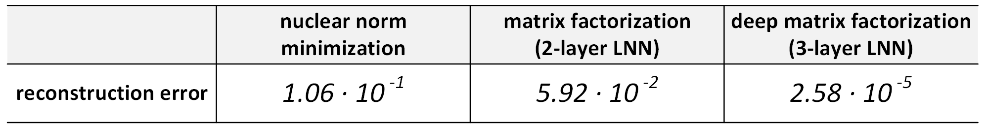
Table 1: Results for matrix completion with small number of observations.
The main focus of our paper is on developing a theoretical understanding of this phenomenon.
Trajectory Analysis: Implicit Regularization Towards Low Rank
We are interested in understanding what end-to-end matrix $W$ emerges when we run GD on an LNN to minimize a general convex loss $L(W)$, and in particular the matrix completion loss given above. Note that $L(W)$ is convex, but the objective obtained by over-parameterizing with an LNN is not. We analyze the trajectories of $W$, and specifically the dynamics of its singular value decomposition. Denote the singular values by $\{ \sigma_r \}_r$, and the corresponding left and right singular vectors by $\{ \mathbf{u}_r \}_r$ and $\{ \mathbf{v}_r \}_r$ respectively.
We start by considering GD applied to $L(W)$ directly (no over-parameterization).
Known result: Minimizing $L(W)$ directly by GD (with small learning rate $\eta$) leads the singular values of $W$ to evolve by: [ \sigma_r(t + 1) \leftarrow \sigma_r(t) - \eta \cdot \langle \nabla L(W(t)) , \mathbf{u}_r(t) \mathbf{v}_r^\top(t) \rangle ~. \qquad (1) ]
This statement implies that the movement of a singular value is proportional to the projection of the gradient onto the corresponding singular component.
Now suppose that we parameterize $W$ with an $N$-layer LNN, i.e. as $W = W_N W_{N-1} \cdots W_1$. In previous work (described in Nadav’s earlier blog post) we have shown that running GD on the LNN, with small learning rate $\eta$ and initialization close to the origin, leads the end-to-end matrix $W$ to evolve by:
\[W(t+1) \leftarrow W(t) - \eta \cdot \sum\nolimits_{j=1}^{N} \left[ W(t) W^\top(t) \right]^\frac{j-1}{N} \nabla{L}(W(t)) \left[ W^\top(t) W(t) \right]^\frac{N-j}{N} ~.\]In the new paper we rely on this result to prove the following:
Theorem: Minimizing $L(W)$ by running GD (with small learning rate $\eta$ and initialization close to the origin) on an $N$-layer LNN leads the singular values of $W$ to evolve by: [ \sigma_r(t + 1) \leftarrow \sigma_r(t) - \eta \cdot \langle \nabla L(W(t)) , \mathbf{u}_r(t) \mathbf{v}_r^\top(t) \rangle \cdot \color{purple}{N \cdot (\sigma_r(t))^{2 - 2 / N}} ~. ]
Comparing this to Equation $(1)$, we see that over-parameterizing the loss $L(W)$ with an $N$-layer LNN introduces the multiplicative factors $\color{purple}{N \cdot (\sigma_r(t))^{2 - 2 / N}}$ to the evolution of singular values. While the constant $N$ does not change relative dynamics (can be absorbed into the learning rate $\eta$), the terms $(\sigma_r(t))^{2 - 2 / N}$ do $-$ they enhance movement of large singular values, and on the hand attenuate that of small ones. Moreover, the enhancement/attenuation becomes more significant as $N$ (network depth) grows.
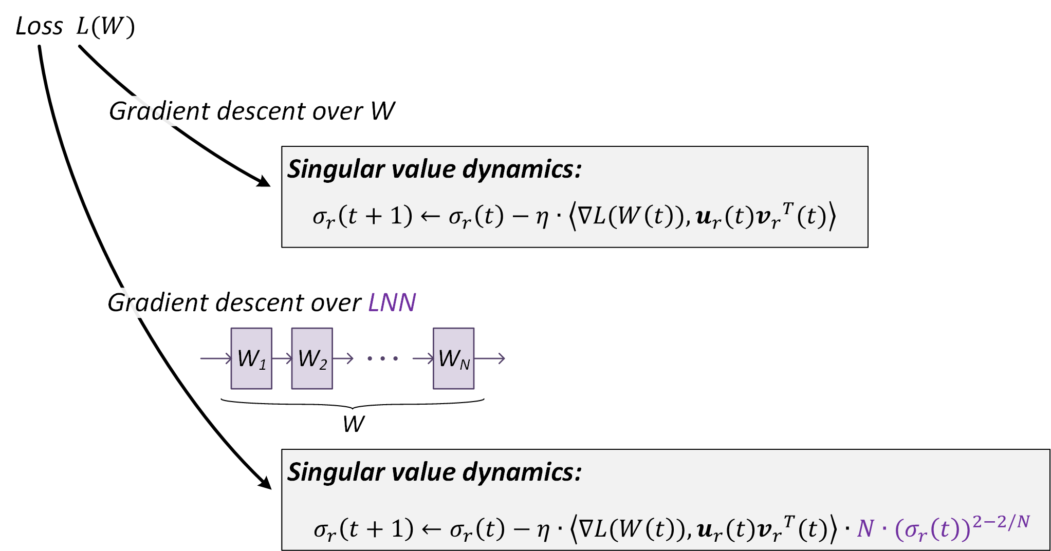
Figure 1: Over-parameterizing with LNN modifies dynamics of singular values.
The enhancement/attenuation effect induced by an LNN (factors $\color{purple}{N \cdot (\sigma_r(t))^{2 - 2 / N}}$) leads each singular value to progress very slowly after initialization, when close to zero, and then, upon reaching a certain threshold, move rapidly, with the transition from slow to rapid movement being sharper in case of a deeper network (larger $N$). If the loss $L(W)$ is underdetermined (has multiple optima) these dynamics promote solutions that have a few large singular values and many small ones (that have yet to reach the phase transition between slow to rapid movement), with a gap that is more extreme the deeper the network is. This is an implicit regularization towards low rank, which intensifies with depth. In the paper we support the intuition with empirical evaluations and theoretical illustrations, demonstrating how adding depth to an LNN can lead GD to produce solutions closer to low-rank. For example, the following plots, corresponding to a task of matrix completion, show evolution of singular values throughout training of networks with varying depths $-$ as can be seen, adding layers indeed admits a final solution whose spectrum is closer to low-rank, thereby improving generalization.
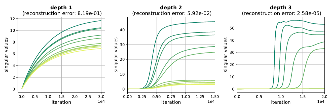
Figure 2: Dynamics of singular values in training matrix factorizations (LNN).
Do the Trajectories Minimize Some Regularized Objective?
In recent years, researchers have come to realize the importance of implicit regularization induced by the choice of optimization algorithm. The strong gravitational pull of the conventional view on optimization (see Sanjeev’s post) has led most papers on this line to try and capture the effect in the language of regularized objectives. For example, it is known that over linear models, i.e. depth $1$ networks, GD finds the solution with minimal Frobenius norm (cf. Section 5 in Zhang et al.), and a common hypothesis is that this persists over more elaborate neural networks, with Frobenius norm potentially replaced by some other norm (or quasi-norm) that depends on network architecture. Gunasekar et al. explicitly conjectured:
Conjecture (by Gunasekar et al., informally stated): GD (with small learning rate and near-zero initialization) training a matrix factorization finds a solution with minimum nuclear norm.
This conjecture essentially states that matrix factorization (i.e. $2$-layer LNN) trained by GD is equivalent to the famous method of nuclear norm minimization. Gunasekar et al. motivated the conjecture with some empirical evidence, as well as mathematical evidence in the form of a proof for a (very) restricted setting.
Given the empirical observation by which adding depth to a matrix factorization can improve results in matrix completion, it would be natural to extend the conjecture of Gunasekar et al., and assert that the implicit regularization with depth $3$ or higher corresponds to minimizing some other norm (or quasi-norm) that approximates rank better than nuclear norm does. For example, a natural candidate would be a Schatten-$p$ quasi-norm with some $0 < p < 1$.
Our investigation began with this approach, but ultimately, we became skeptical of the entire “implicit regularization as norm minimization” line of reasoning, and in particular of the conjecture by Gunasekar et al.
Theorem (mathematical evidence against the conjecture): In the same restricted setting for which Gunasekar et al. proved their conjecture, nuclear norm is minimized by GD over matrix factorization not only with depth $2$, but with any depth $\geq 3$ as well.
This theorem disqualifies Schatten quasi-norms as the implicit regularization in deep matrix factorizations, and instead suggests that all depths correspond to nuclear norm. However, empirically we found a notable difference in performance between different depths, so the conceptual leap from a proof in the restricted setting to a general conjecture, as done by Gunasekar et al., seems questionable.
In the paper we conduct a systematic set of experiments to empirically evaluate the conjecture. We find that in the regime where nuclear norm minimization is suboptimal (few observed entries), matrix factorizations consistently outperform it (see for example Table 1). This holds in particular with depth $2$, in contrast to the conjecture’s prediction. Together, our theory and experiments lead us to believe that it may not be possible to capture the implicit regularization in LNN with a single mathematical norm (or quasi-norm).
Full details behind our results on “implicit regularization as norm minimization” can be found in Section 2 of the paper. The trajectory analysis we discussed earlier appears in Section 3 there.
Conclusion
The conventional view of optimization has been integral to the theory of machine learning. Our study suggests that the associated vocabulary may not suffice for understanding generalization in deep learning, and one should instead analyze trajectories of optimization, taking into account that speed of convergence does not necessarily correlate with generalization. We hope this work will motivate development of a new vocabulary for analyzing deep learning.