This blog post concerns our ICLR20 paper on a surprising discovery about learning rate (LR), the most basic hyperparameter in deep learning.
As illustrated in many online blogs, setting LR too small might slow down the optimization, and setting it too large might make the network overshoot the area of low losses. The standard mathematical analysis for the right choice of LR relates it to smoothness of the loss function.
Many practitioners use a ‘step decay’ LR schedule, which systematically drops the LR after specific training epochs. One often hears the intuition—with some mathematical justification if one treats SGD as a random walk in the loss landscape— that large learning rates are useful in the initial (“exploration”) phase of training whereas lower rates in later epochs allow a slow settling down to a local minimum in the landscape. Intriguingly, this intuition is called into question by the success of exotic learning rate schedules such as cosine (Loshchilov&Hutter, 2016), and triangular (Smith, 2015), featuring an oscillatory LR. These divergent approaches suggest that LR, the most basic and intuitive hyperparameter in deep learning, has not revealed all its mysteries yet.
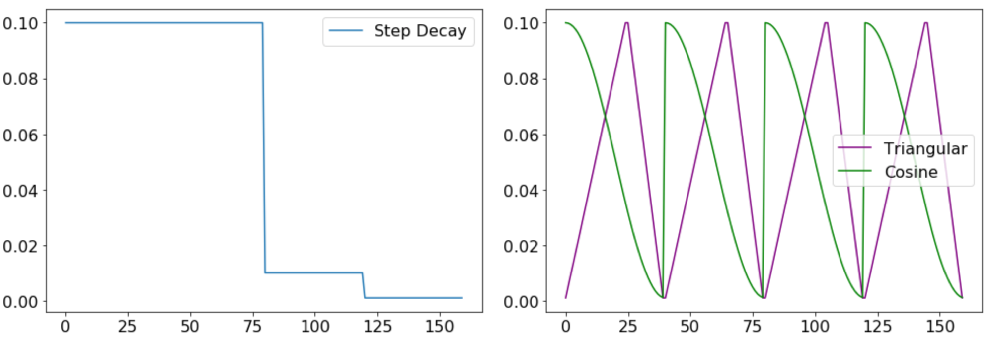
Figure 1. Examples of Step Decay, Triangular and Cosine LR schedules.
Surprise: Exponentially increasing LR
We report experiments that state-of-the-art networks for image recognition tasks can be trained with an exponentially increasing LR (ExpLR): in each iteration it increases by $(1+\alpha)$ for some $\alpha > 0$. (The $\alpha$ can be varied over epochs.) Here $\alpha$ is not too small in our experiments, so as you would imagine, the LR hits astronomical values in no time. To the best of our knowledge, this is the first time such a rate schedule has been successfully used, let alone for highly successful architectures. In fact, as we will see below, the reason we even did this bizarre experiment was that we already had a mathematical proof that it would work. Specifically, we could show that such ExpLR schedules are at least as powerful as the standard step-decay ones, by which we mean that ExpLR can let us achieve (in function space) all the nets obtainable via the currently popular step-decay schedules.
So why does this work?
One key property of state-of-the-art nets we rely on is that they all use some normalization of parameters within layers, usually Batch Norm (BN), which has been shown to give benefits in optimization and generalization across architectures. Our result also holds for other normalizations, including Group Normalization (Wu & He, 2018), Layer Normalization (Ba et al., 2016), Instance Norm (Ulyanov et al., 2016), etc.
The second key property of current training is that they use weight decay (aka $\ell_2$ regularizer). When combined with BN, this implies strange dynamics in parameter space, and the experimental papers (van Laarhoven, 2017, Hoffer et al., 2018a and Zhang et al., 2019), noticed that combining BN and weight decay can be viewed as increasing the LR.
Our paper gives a rigorous proof of the power of ExpLR by showing the following about the end-to-end function being computed (see Main Thm in the paper):
(Informal Theorem) For commonly used values of the paremeters, every net produced by Weight Decay + Constant LR + BN + Momentum can also be produced (in function space) via ExpLR + BN + Momentum
*NB: If the LR is not fixed but decaying in discrete steps, then the equivalent ExpLR training decays the exponent. (See our paper for details.)
At first sight such a claim may seem difficult (if not impossible) to prove given that we lack any mathematical characterization of nets produced by training (note that the theorem makes no mention of the dataset!). The equivalence is shown by reasoning about trajectory of optimization, instead of the usual “landscape view” of stationary points, gradient norms, Hessian norms, smoothness, etc.. This is an example of the importance of trajectory analysis, as argued in earlier blog post of Sanjeev’s because optimization and generalization are deeply intertwined for deep learning. Conventional wisdom says LR controls optimization, and the regularizer controls generalization. Our result shows that the effect of weight decay can under fairly normal conditions be * exactly* realized by the ExpLR rate schedule.
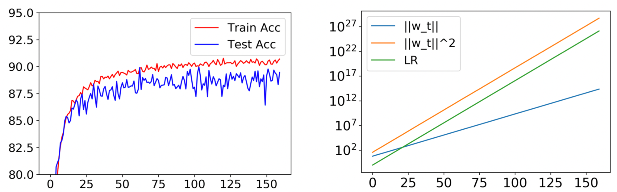
Figure 2. Training PreResNet32 on CIFAR10 with fixed LR $0.1$, momentum $0.9$ and other standard hyperparameters. Trajectory was unchanged when WD was turned off and LR at iteration $t$ was $\tilde{\eta}_ t = 0.1\times1.481^t$. (The constant $1.481$ is predicted by our theory given the original hyperparameters.) Plot on right shows weight norm $\pmb{w}$ of the first convolutional layer in the second residual block. It grows exponentially as one would expect, satisfying $|\pmb{w}_ t|_ 2^2/\tilde{\eta}_ t = $ constant.
Scale Invariance and Equivalence
The formal proof holds for any training loss satisfying what we call Scale Invariance:
\[L (c\cdot \pmb{\theta}) = L(\pmb{\theta}), \quad \forall \pmb{\theta}, \forall c >0.\]BN and other normalization schemes result in a Scale-Invariant Loss for the popular deep architectures (Convnet, Resnet, DenseNet etc.) if the output layer –where normally no normalization is used– is fixed throughout training. Empirically, Hoffer et al. (2018b) found that randomly fixing the output layer at the start does not harm the final accuracy. (Appendix C of our paper demonstrates scale invariance for various architectures; it is somewhat nontrivial.)
For batch ${\mathcal{B}} = \{ x_ i \} _ {i=1}^B$, network parameter ${\pmb{\theta}}$, we denote the network by $f_ {\pmb{\theta}}$ and the loss function at iteration $t$ by $L_ t(f_ {\pmb{\theta}}) = L(f_ {\pmb{\theta}}, {\mathcal{B}}_ t)$ . We also use $L_ t({\pmb{\theta}})$ for convenience. We say the network $f_ {\pmb{\theta}}$ is scale invariant if $\forall c>0$, $f_ {c{\pmb{\theta}}} = f_ {\pmb{\theta}}$, which implies the loss $L_ t$ is also scale invariant, i.e., $L_ t(c{\pmb{\theta}}_ t)=L_ t({\pmb{\theta}}_ t)$, $\forall c>0$. A key source of intuition is the following lemma provable via chain rule:
Lemma 1. A scale-invariant loss $L$ satisfies (1). $\langle\nabla_ {\pmb{\theta}} L, {\pmb{\theta}} \rangle=0$ ;
(2). $\left.\nabla_ {\pmb{\theta}} L \right|_ {\pmb{\theta} = \pmb{\theta}_ 0} = c \left.\nabla_ {\pmb{\theta}} L\right|_ {\pmb{\theta} = c\pmb{\theta}_ 0}$, for any $c>0$.
The first property immediately implies that $|{\pmb{\theta}}_ t|$ is monotone increasing for SGD if WD is turned off by Pythagoren Theorem. And based on this, our previous work with Kaifeng Lyu shows that GD with any fixed learning rate can reach $\varepsilon$ approximate stationary point for scale invariant objectives in $O(1/\varepsilon^2)$ iterations.
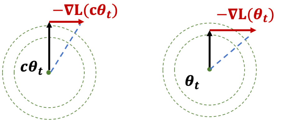
Figure 3. Illustration of Lemma 1.
Below is the main result of the paper. We will explain the proof idea (using scale-invariance) in a later post.
Theorem 1(Main, Informal). SGD on a scale-invariant objective with initial learning rate $\eta$, weight decay factor $\lambda$, and momentum factor $\gamma$ is equivalent to SGD with momentum factor $\gamma$ where at iteration $t$, the ExpLR $\tilde{\eta}_ t$ is defined as $\tilde{\eta}_ t = \alpha^{-2t-1} \eta$ without weight decay($\tilde{\lambda} = 0$) where $\alpha$ is a non-zero root of equation \(x^2-(1+\gamma-\lambda\eta)x + \gamma = 0,\)
Specifically, when momentum $\gamma=0$, the above schedule can be simplified as $\tilde{\eta}_ t = (1-\lambda\eta)^{-2t-1} \eta$.
SOTA performance with exponential LR
As mentioned, reaching state-of-the-art accuracy requires reducing the learning rate a few times. Suppose the training has $K$ phases, and the learning rate is divided by some constant $C_I>1$ when entering phase $I$. To realize the same effect with an exponentially increasing LR, we have:
Theorem 2: ExpLR with the below modification generates the same network sequence as Step Decay with momentum factor $\gamma$ and WD $\lambda$ does. We call it Tapered Exponential LR schedule (TEXP).
Modification when entering a new phase $I$: (1). switching to some smaller exponential growing rate; (2). divinding the current LR by $C_I$.
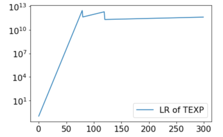
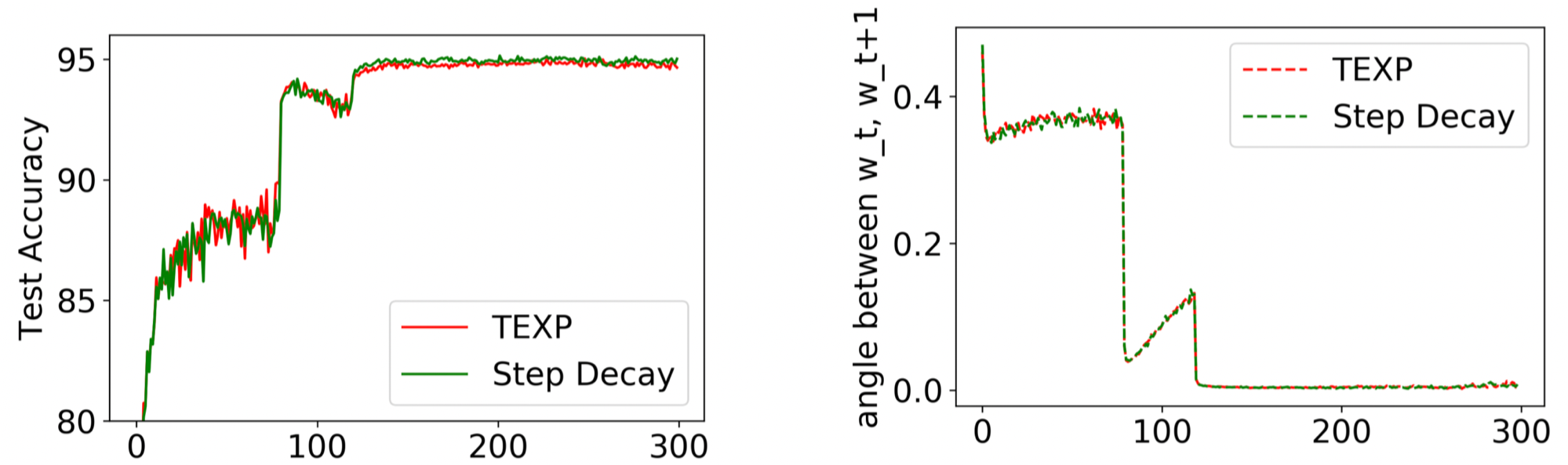
Figure 5. PreResNet32 trained with Step Decay (as in Figure 1) and its corresponding TEXP schedule. As predicted by Theorem 2, they have similar trajectories and performances.
Conclusion
We hope that this bit of theory and supporting experiments have changed your outlook on learning rates for deep learning.
A follow-up post will present the proof idea and give more insight into why ExpLR suggests a rethinking of the “landscape view” of optimization in deep learning.