GANs, originally discovered in the context of unsupervised learning, have had far reaching implications to science, engineering, and society. However, training GANs remains challenging (in part) due to the lack of convergent algorithms for nonconvex-nonconcave min-max optimization. In this post, we present a new first-order algorithm for min-max optimization which is particularly suited to GANs. This algorithm is guaranteed to converge to an equilibrium, is competitive in terms of time and memory with gradient descent-ascent and, most importantly, GANs trained using it seem to be stable.
GANs and min-max optimization
Starting with the work of Goodfellow et al., Generative Adversarial Nets (GANs) have become a critical component in various ML systems; for prior posts on GANs, see here for a post on GAN architecture, and here and here for posts which discuss some of the many difficulties arising when training GANs.
Mathematically, a GAN consists of a generator neural network $\mathcal{G}$ and a discriminator neural network $\mathcal{D}$ that are competing against each other in a way that, together, they learn the unknown distribution from which a given dataset arises. The generator takes a random “noise” vector as input and maps this vector to a sample; for instance, an image. The discriminator takes samples – “fake” ones produced by the generator and “real” ones from the given dataset – as inputs. The discriminator then tries to classify these samples as “real” or “fake”. As a designer, we would like the generated samples to be indistinguishable from those of the dataset. Thus, our goal is to choose weights $x$ for the generator network that allow it to generate samples which are difficult for any discriminator to tell apart from real samples. This leads to a min-max optimization problem where we look for weights $x$ which minimize the rate (measured by a loss function $f$) at which any discriminator correctly classifies the real and fake samples. And, we seek weights $y$ for the discriminator network which maximize this rate.
Min-max formulation of GANs
\[\min_x \max_y f(x,y),\] \[f(x,y) := \mathbb{E}[ f_{\zeta, \xi}(x,y)],\]
where $\zeta$ is a random sample from the dataset, and $\xi \sim N(0,I_d)$ is a noise vector which the generator maps to a “fake” sample. $f_{\zeta, \xi}$ measures how accurately the discriminator $\mathcal{D}(y;\cdot)$ distinguishes $\zeta$ from $\mathcal{G}(x;\xi)$ produced by the generator using the input noise $\xi$.
In this formulation, there are several choices that we have to make as a GAN designer, and an important one is that of a loss function. One concrete choice is from the paper of Goodfellow et al.: the cross-entropy loss function:
\[f_{\zeta, \xi}(x,y) := \log(\mathcal{D}(y;\zeta)) + \log(1-\mathcal{D}(y;\mathcal{G}(x;\xi)))\]See here for a summary and comparison of different loss functions.
Once we fix the loss function (and the architecture of the generator and discriminator), we can compute unbiased estimates of the value of $f$ and its gradients $\nabla_x f$ and $\nabla_y f$ using batches consisting of random Gaussian noise vectors $\xi_1,\ldots, \xi_n \sim N(0,I_d)$ and random samples from the dataset $\zeta_1, \ldots, \zeta_n$. For example, the stochastic batch gradient
\[\frac{1}{n} \sum_{i=1}^n \nabla_x f_{\zeta_i, \xi_i}(x,y)\]gives us an unbiased estimate for $\nabla_x f(x,y)$.
But how do we solve the min-max optimization problem above using such a first-order access to $f$?
Gradient descent-ascent and variants
Perhaps the simplest algorithm we can try for min-max optimization is gradient descent-ascent (GDA). As the generator wants to minimize with respect to $x$ and the discriminator wants to maximize with respect to $y$, the idea is to do descent steps for $x$ and ascent steps for $y$. How exactly to do this is not clear, and one strategy is to let the generator and discriminator alternate:
\[x_{i+1} = x_i -\nabla_x f(x_i,y_i),\] \[y_{i+1} = y_i +\nabla_y f(x_i,y_i).\]Other variants include, for instance, optimistic mirror descent (OMD) (see also here and here for applications of OMD to GANs, and here for an analysis of OMD and related methods)
\[x_{i+1} = x_i -2\nabla_x f(x_i,y_i) + \nabla_x f(x_{i-1},y_{i-1})\] \[y_{i+1} = y_i +2\nabla_y f(x_i,y_i)- \nabla_y f(x_{i-1},y_{i-1}).\]The advantage of such algorithms is that they are quite practical. The problem, as we discuss next, is that they are not always guaranteed to converge. Most of these guarantees only hold for special classes of loss functions $f$ that satisfy properties such as concavity (see here and here) or monotonicity, or under the assumptions that these algorithms are provided with special starting points (see here, here).
Convergence problems with current algorithms
Unfortunately there are simple functions for which some min-max optimization algorithms may never converge to any point. For instance GDA may not converge on $f(x,y) = xy$ (see Figure 1, and our previous post for a more detailed discussion).

Figure 1. GDA on $f(x,y) = xy, \, \, \, \, x,y \in [-5,5]$ (the red line is the set of global min-max points). GDA is non-convergent from almost every initial point.
As for examples relevant to ML, when using GDA to train a GAN on a dataset consisting of points sampled from a mixture of four Gaussians in $\mathbb{R}^2$, we observe that GDA tends to cause the generator to cycle between different modes corresponding to the four Gaussians. We also used GDA to train a GAN on the subset of the MNIST digits which have “0” or “1” as their label, which we refer to as the 0-1 MNIST dataset. We observed a cycling behavior for this dataset as well: After learning how to generate images of $0$’s, the GAN trained by GDA then forgets how to generate $0$’s for a long time and only generates $1$’s.
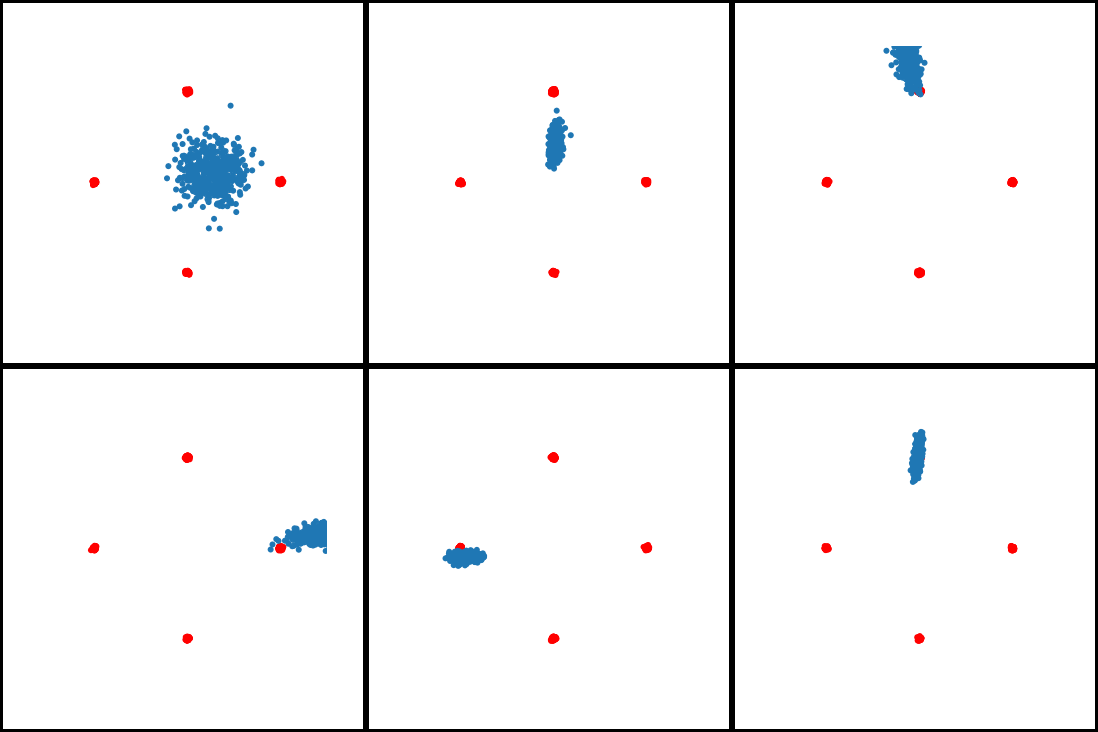
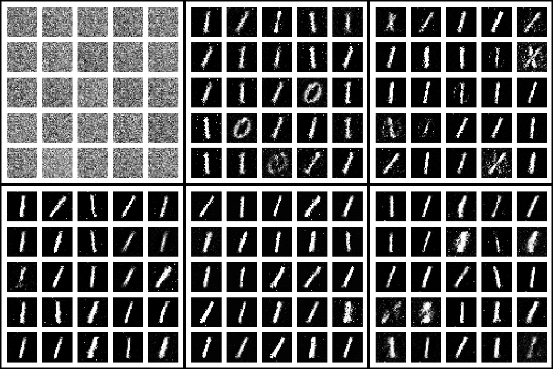
Figure 2. Mode oscillation when GDA is used to train GANs on the four Guassian mixture dataset (left) and the 0-1 MNIST dataset (right).
In algorithms such as GDA where the discriminator only makes local updates, cycling can happen for the following reason: Once the discriminator learns to identify one of the modes (say mode “A”), the generator can update $x$ in a way that greatly decreases f, by (at least temporarily) ìfoolingî the discriminator. The generator does this by learning to generate samples from a different mode (say mode “B”) which the discriminator has not yet learned to identify, and stops generating samples from mode A. However, after many iterations, the discriminator ìcatches upî to the generator and learns how to identify mode B. Since the generator is no longer generating samples from mode A, the discriminator may then ìforgetî how to identify samples from this mode. And this can cause the generator to switch back to generating only mode A.
Our first-order algorithm
To solve the min-max optimization problem, at any point $(x,y)$, we should ideally allow the discriminator to find the global maximum, $\max_z f(x,z)$. However, this may be hard for nonconcave $f$. But we could still let the discriminator run a convergent algorithm (such as gradient ascent) until it reaches a first-order stationary point, allowing it to compute an approximation $h$ for the global max function. (Note that even though $\max_z f(x,z)$ is only a function of $x$, since $h$ is a “local’’ approximation it could also depend on the initial point $y$ where we start gradient ascent.) And we also empower the generator to simulate the discriminator’s update by running gradient ascent (see our paper for discriminators with access to a more general class of first-order algorithms).
Idea 1: Use a local approximation to global max
Starting at the point $(x,y)$, update $y$ by computing multiple gradient ascent steps for $y$ until a point $w$ is reached where \(\|\nabla_y f(x,w)\|\) is close to zero and define $h(x,y) := f(x,w)$.
We would like the generator to minimize $h(\cdot,y)$. To minimize $h$, we would ideally like to update $x$ in the direction $-\nabla_x h$. However, $h$ may be discontinuous in $x$ (see our previous post for why this can happen). Moreover, even at points where $h$ is differentiable, computing the gradient of $h$ can take a long time and requires a large amount of memory.
Thus, realistically, we only have access to the value of $h$. A naive approach to minimizing $h$ would be to propose a random update to $x$, for instance an update sampled from a standard Gaussian, and then only accept this update if it causes the value of $h$ to decrease. Unfortunately, this does not lead to fast algorithms as even at points where $h$ is differentiable, in high dimensions, a random Gaussian step will be almost orthogonal to the steepest descent direction $-\nabla_x h(x,y)$, making the progress slow.
Another idea is to have the generator propose at each iteration an update in the direction of the gradient $-\nabla_x f(x,y)$, and to then have the discriminator update $y$ using gradient ascent. To see why this may be a reasonable thing to do, notice that once the generator proposes an update $v$ to $x$, the discriminator will only make updates which increase the value of f or, $h(x+v,y) \geq f(x+v,y)$. And, since $y$ is a first-order stationary point for $f(x, \cdot)$ (because $y$ was computed using gradient ascent in the previous iteration), we also have that $h(x,y)=f(x,y)$. Hence,
\[f(x+v,y) \leq h(x+v,y) < h(x,y) = f(x,y).\]This means that decreasing $h$ requires us to decrease $f$ (the converse is not true). So it indeed makes sense to move in the direction $-\nabla_x f(x,y)$!
While making updates using $-\nabla_x f(x,y)$ may allow the generator to decrease $h$ more quickly than updating in a random direction, it is not always the case that updating in the direction of $-\nabla_x f$ will lead to a decrease in $h$ (and doing so may even lead to an increase in $h$!). Instead, our algorithm has the generator perform a random search by proposing an update in the direction of a batch gradient with mean $-\nabla_x f$, and accepts this move only if the value of $h$ (the local approximation) decreases. The accept-reject step prevents our algorithm from cycling between modes, and using the batch gradient for the random search allows our algorithm to be competitive with prior first-order methods in terms of running time.
Idea 2: Use zeroth-order optimization with batch gradients
Sample a batch gradient $v$ with mean $-\nabla_x f(x,y)$.
If $h(x+ v, y) < h(x,y) $ accept the step $x+v$; otherwise reject it.
A final issue, that applies even in the special case of minimization, is that converging to a local minimum point does not mean that point is desirable from an application standpoint. The same is true for the more general setting of min-max optimization. To help our algorithm escape undesirable local min-max equilibria, we use a randomized accept-reject rule inspired by simulated annealing. Simulated annealing algorithms seek to minimize a function via a randomized search, while gradually decreasing the acceptance probability of this search; in some cases this allows one to reach the global minimum of a nonconvex function (see for instance this paper). These three ideas lead us to our algorithm.
Our algorithm
Input: Initial point $(x,y)$, $f: \mathbb{R}^d \times \mathbb{R}^d\rightarrow \mathbb{R}$
Output: A local min-max equilibrium $(x,y)$
For $i = 1,2, \ldots$
Step 1: Generate a batch gradient $v$ with mean $-\nabla_x f(x,y)$ and propose the generator update $x+v$.
Step 2: Compute $h(x+v, y) = f(x+v, w)$, by simulating a discriminator update $w$ via gradient ascent on $f(x+v, \cdot)$ starting at $y$.
Step 3: If $h(x+v, y)$ is less than $h(x,y) = f(x,y)$, accept both updates: $(x,y) = (x+v, w)$. Else, accept both updates with some small probability.
In our paper, we show that our algorithm is guaranteed to converge to a type of local min-max equilibrium in $\mathrm{poly}(\frac{1}{\varepsilon},d, b, L)$ time whenever $f$ is bounded by some $b>0$ and has $L$-Lipschitz gradients. Our algorithm does not require any special starting points, or any additional assumptions on $f$ such as convexity or monotonicity. (See Definition 3.2 and Theorem 3.3 in our paper.)

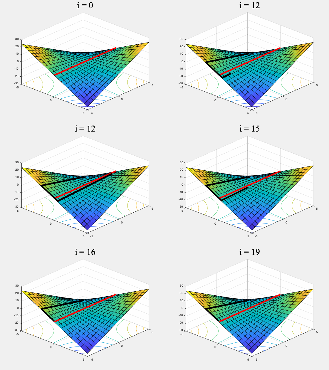
Figure 3. GDA (left) and a version of our algorithm (right) on $f(x,y) = xy, \, \, \, \, x,y \in [-5,5]$. While GDA is non-convergent from almost every initial point, our algorithm converges to the set of global min-max points (the red line). To ensure it converges to a (local) equilibrium, our algorithm's generator proposes multiple updates, simulates the discriminator's response, and rejects updates which do not lead to a net decrease in $f$. It only stops if it can't find such an update after many attempts. (To stay inside $[-5,5]\times [-5,5]$ this version of our algorithm uses projected gradients.)
So, how does our algorithm perform in practice?
When training a GAN on the mixture of four Gaussians dataset, we found that our algorithm avoids the cycling behavior observed in GDA. We ran each algorithm multiple times, and evaluated the results visually. By the 1500’th iteration GDA learned only one mode in 100% of the runs, and tended to cycle between two or more modes. In contrast, our algorithm was able to learn all four modes 68% of the runs, and three modes 26% of the runs.
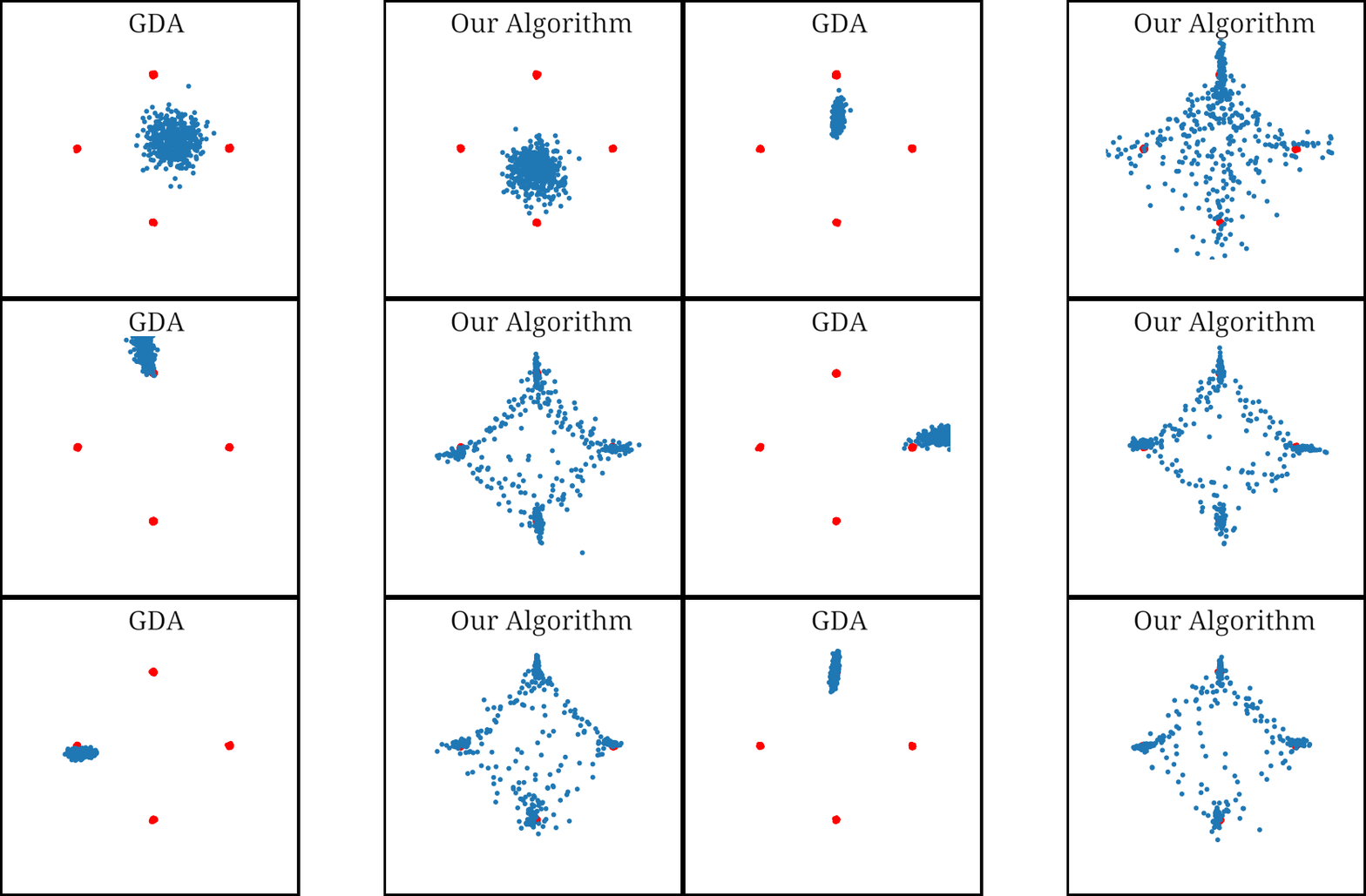
Figure 4. GAN trained using GDA and our algorithm on a four Gaussian mixture dataset. While GDA cycles between the Gaussian modes (red dots), our algorithm learns all four modes.
When training on the 0-1 MNIST dataset, we found that GDA tends to briefly generate shapes that look like a combination of $0$’s and $1$’s, then switches to generating only $1$’s, and then re-learns how to generate $0$’s. In contrast, our algorithm seems to learn how to generate both $0$’s and $1$’s early on and does not stop generating either digit. We repeated this simulation multiple times for both algorithms, and visually inspected the images at the 1000’th iteration. GANs trained using our algorithm generated both digits by the 1000’th iteration in 86% of the runs, while those trained using GDA only did so in 23% of the runs.
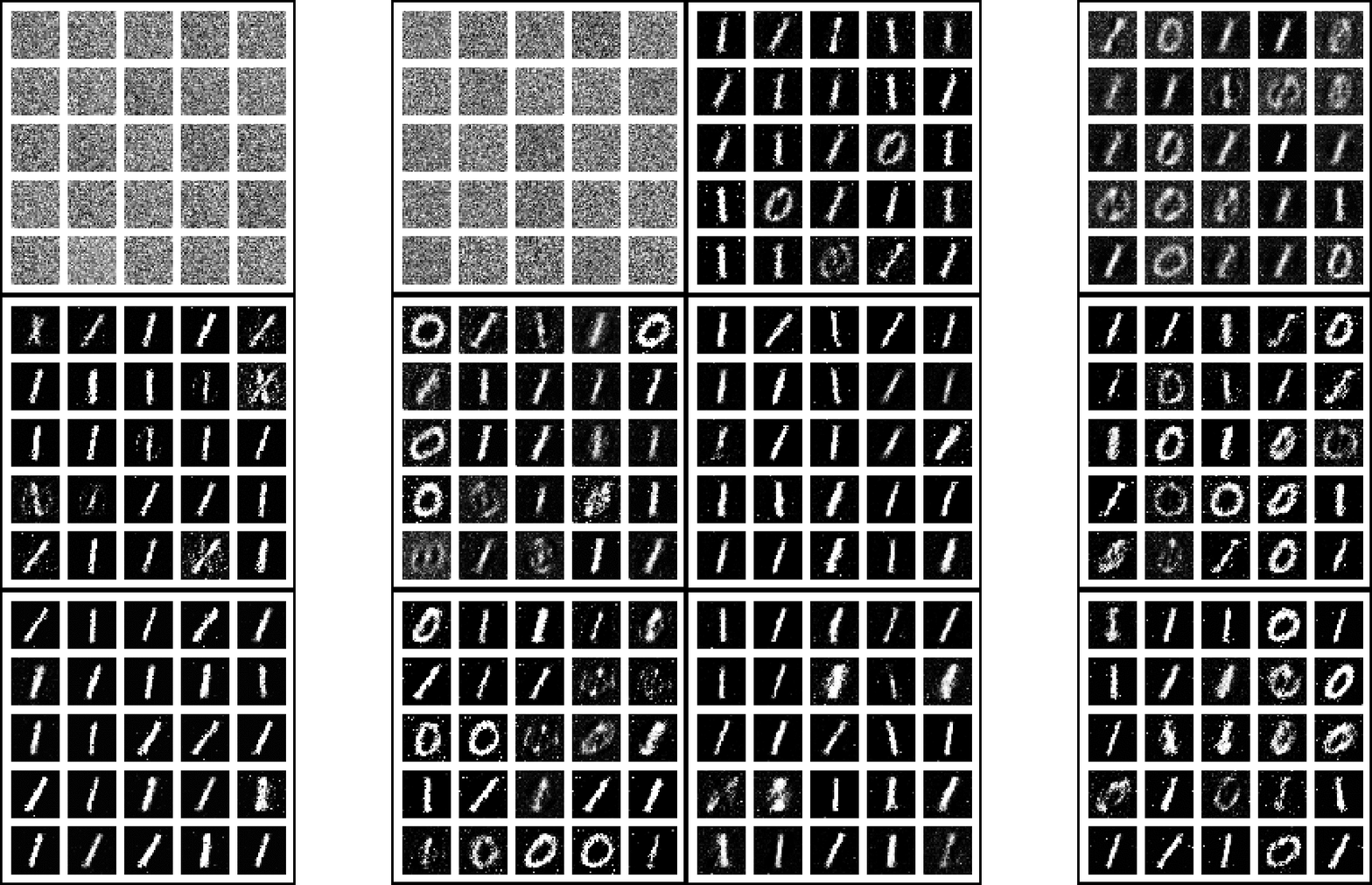
Figure 5. We trained a GAN with GDA and our algorithm on the 0-1 MNIST dataset. During the first 1000 iterations, GDA (left) forgets how to generate $0$'s, while our algorithm (right) learns how to generate both $0$'s and $1$'s early on and does not stop generating either digit.
While here we have focused on comparing our algorithm to GDA, in our paper we also include a comparison to Unrolled GANs, which exhibits cycling between modes. We also present results for CIFAR-10 (see Figures 3 and 7 in our paper), where we compute FID scores to track the progress of our algorithm. See our paper for more details; the code is available on GitHub.
Conclusion
In this post we have shown how to develop a practical and convergent first-order algorithm for training GANs. Our algorithm synthesizes an approximation to the global max function based on first-order algorithms, random search using batch gradients, and simulated annealing. Our simulations show that a version of this algorithm can lead to more stable training of GANs. And yet the amount of memory and time required by each iteration of our algorithm is competitive with GDA. This post, together with the previous post, show that different local approximations to the global max function $\max_z f(x,z)$ can lead to different types of convergent algorithms for min-max optimization. We believe that this idea should be useful in other applications of min-max optimization.
