As the growing number of posts on this blog would suggest, recent years have seen a lot of progress in understanding optimization beyond convexity. However, optimization is only one of the basic algorithmic primitives in machine learning — it’s used by most forms of risk minimization and model fitting. Another important primitive is sampling, which is used by most forms of inference (i.e. answering probabilistic queries of a learned model).
It turns out that there is a natural analogue of convexity for sampling — log-concavity. Paralleling the state of affairs in optimization, we have a variety of (provably efficient) algorithms for sampling from log-concave distributions, under a variety of access models to the distribution. Log-concavity, however, is very restrictive and cannot model common properties of distributions we frequently wish to sample from in machine learning applications, for example multi-modality and manifold structure in the level sets, which is what we’ll focus on in this and the upcoming post.
Unlike non-convex optimization, the field of sampling beyond log-concavity is very nascent. In this post, we will survey the basic tools and difficulties for sampling beyond log-concavity. In the next post, we will survey recent progress in this direction, in particular with respect to handling multi-modality and manifold structure in the level sets, covering the papers Simulated tempering Langevin Monte Carlo by Rong Ge, Holden Lee, and Andrej Risteski and Fast convergence for Langevin diffusion with matrix manifold structure by Ankur Moitra and Andrej Risteski.
Formalizing the sampling problem
The formulation of the sampling problem we will consider is as follows:
Problem: Sample from a distribution $p(x) \propto e^{-f(x)}$ given black-box access to $f$ and $\nabla f$.
This formalization subsumes a lot of inference tasks involving different kinds of probabilistic models. We give several common examples:
1.Posterior inference: Suppose our data is generated from a model with unknown parameters $\theta$ , such that the data-generation process is given by $p(x \mid \theta)$ and we have a prior $p(\theta)$ over the model parameters. Then the posterior distribution $p(\theta \mid x)$ , by Bayes’s Rule, is given by
\[p(\theta \mid x) = \frac{p(x \mid \theta)p(x)}{p(x)}\propto p(x \mid \theta)p(\theta).\]A canonical example of this is a noisy inference task where a signal (parametrized by $\theta$ ) is perturbed by noise (as specified by $p(x \mid \theta)$ ).
2.Posteriors in latent-variable models: If the data-generation process has a latent (hidden) variable $h$ associated to each data point, such that $h$ has a known prior $p(h)$ and a known conditional $p_\theta(x \mid h)$ , then again by Bayes’s rule, we have
\[p_\theta(h \mid x) = \frac{p_\theta(x \mid h)p_\theta(h)}{p_\theta(x)}\propto p_\theta(x \mid h)p_\theta(h).\]In typical latent-variable models, $p_\theta(x \mid h)$ and $p_\theta(h)$ have a simple parametric form, which makes it easy to evaluate $p_\theta(x \mid h)p_\theta(h)$ . Some examples of latent-variable models are mixture models (where $h$ encodes which component a sample came from), topic models (where $h$ denote the topic proportions in a document), and noisy-OR networks (and latent-variable Bayesian belief networks).
3.Sampling from energy models: in energy models, the distribution of the data is parametrized as $p(x) \propto \exp(-E(x))$ for some energy function $E(x)$ which is smaller on points in the data distribution. Recent works by (Song, Ermon 2019) and (Du, Mordatch 2019) have scaled up the training of these models on images so that the visual quality of the samples they produce is comparable to that of more popular generative models like GANs and flow models.
The “exponential form” $e^{-f(x)}$ is also helpful in making an analogy to optimization. Namely, if we sample from $p(x)\propto e^{-f(x)}$, a particular point $x$ is more likely to be sampled if $f(x)$ is small. The key difference between with optimization is that while in optimization, we only want to get to the minimum, in sampling, we want to pick points with the correct probabilities.
Comparison with optimization
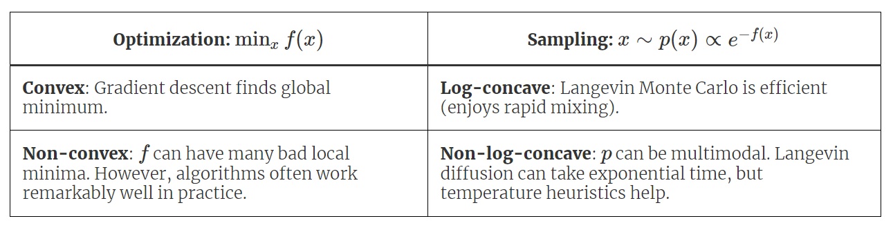
The computational hardness landscape for our sampling problem parallels the one for black-box optimization, in which the goal is to find the minimum of a function $f$, given value/gradient oracle access. When $f$ is convex, there is a unique local minimum, so that local search algorithms like gradient descent are efficient. When $f$ is non-convex, gradient descent can get trapped in potentially poor local minima, and in the worst case, an exponential number of queries is needed.
Similarly, for sampling, when $p$ is log-concave, the distribution is unimodal and a Markov Chain which is a close relative of gradient descent — Langevin Monte Carlo — is efficient. When $p$ is non-log-concave, Langevin Monte Carlo can get trapped in one of many modes, and and exponential number of queries may also be needed.
A distribution $p(x)\propto e^{-f(x)}$ is log-concave if $f(x) = -\log p(x)$ is convex. It is $\alpha$-strongly log-concave if $f(x)$ is $\alpha$-strongly convex.
However, such worst-case hardness rarely stop practitioners from trying to solve the non-convex optimization or non-log-concave sampling problems which are ubiquitous in modern machine learning. Often they manage to do so with great success - for instance, in training deep neural networks, gradient descent and its relatives perform quite well. Similarly, Langevin Monte Carlo and its relatives can do quite well on non-log-concave problems, though they sometimes need to be aided by temperature heuristics and other tricks.
As theorists, we’d like to develop theory that will lead to a better understanding of why and when these heuristics work. Just like we’ve done for optimization, we need to be guided both by hardness results and relevant structure of real-world problems in this endeavour.
The following table summarizes the comparisons we have come up with:
Before we move on to non-log-concave distributions, though, we need to understand the basic algorithm for sampling and its guarantees for log-concave distributions.
Langevin Monte Carlo
Just as gradient descent is the canonical algorithm for optimization, Langevin Monte Carlo (LMC) is the canonical algorithm for our sampling problem. In a nutshell, it is gradient descent that also injects Gaussian noise:
\[\text{Gradient descent:}\quad x_{t+\eta} = x_t - \eta \nabla f(x_t)\] \[\text{Langevin Monte Carlo:}\quad x_{t+\eta} = x_t - \eta \nabla f(x_t) + \sqrt{2\eta}\xi_t,\quad \xi_t\sim N(0,I)\]Both of these processes can be considered as discretizations of a continuous process. For gradient descent, the limit is an ordinary differential equation, and for Langevin Monte Carlo a stochastic differential equation:
\[\text{Gradient flow:} \quad dx_t = -\nabla f(x_t) dt\] \[\text{Langevin diffusion:} \quad dx_t = -\nabla f(x_t) dt + \sqrt{2} dB_t\]where $B_t$ denotes Brownian motion of the appropriate dimension.
The crucial property of the above stochastic differential equation is that under fairly mild assumptions on $f$, the stationary distribution is $p(x) \propto e^{-f(x)}$. (If you’re more comfortable with optimization, note that while gradient descent generally converges to (local) minima, the Gaussian noise term prevents LMC from converging to a single point - rather, it converges to a stationary distribution. See animation below.)
Langevin Monte Carlo fits in the Markov Chain Monte Carlo (MCMC) paradigm: design a random walk, so that the stationary distribution is the desired distribution. “Mixing” means getting close to the stationary distribution, and rapid mixing means this happens quickly.
Like in optimization, Langevin Monte Carlo is the most “basic” algorithm: for example, one can incorporate “acceleration” and obtain underdamped Langevin, or use the physics-inspired Hamiltonian Monte Carlo.
Tools for bounding mixing time, challenges beyond log-concavity
To illustrate the difficulty in moving beyond log-concavity, we’ll describe the tools that are used to prove fast mixing for log-concave distributions, and where they fall short for non-log-concave distributions.
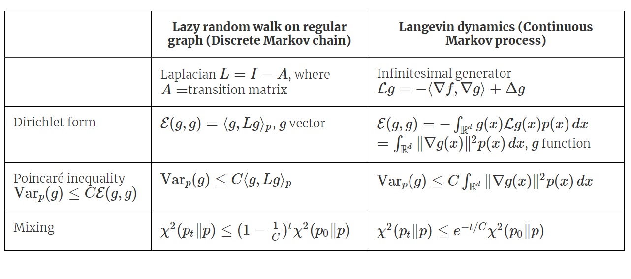
We will do this by an analogy to how we analyze random walks on graphs. One common way to prove rapid mixing of a random walk on a graph is to show the Laplacian has a spectral gap (equivalently, the transition matrix has a gap between the largest and next-to-largest eigenvalue). The analogue of this for Langevin diffusion is showing a Poincaré inequality. (A spectral gap of $1/C$ corresponds to Poincaré constant of $C$.)
We say that $p(x)$ satisfies a Poincaré inequality with constant $C$ if for all functions $g$ on $\mathbb R^d$ (such that $g$ and $\nabla g$ are square-integrable with respect to $p$),
$$\text{Var}_p(g) \le C \int_{\mathbb R^d} ||\nabla g(x)||^2 p(x)\,dx.$$
A small constant $C$ implies fast mixing in $\chi^2$ divergence, which implies fast mixing in total variation distance. More precisely, the mixing time for Langevin diffusion is on the order of $C$. We note that other functional inequalities imply mixing with respect to other measures (such as log-Sobolev inequalities for KL divergence).
While it may not be obvious what the Poincaré inequality has to do with a spectral gap, it turns out that we can think of the right-hand side as a quadratic form involving the infinitesimal generator of Langevin process, which functions as the continuous analogue of a Laplacian for a graph random walk.
The following table shows the analogy: we can put the discrete and continuous processes on the same footing by defining a quadratic form called the Dirichlet form from the Laplacian or infinitesimal generator.
To see how the Poincaré inequality represents a spectral gap in the discrete case, we write it in a more explicit form in a familiar special case: a lazy random walk (i.e. a random walk that with probability $1/2$ stays in the current vertex, and with probability $1/2$ goes to a random neighbor) on a regular graph with $n$ vertices. In this case, $p$ is the uniform distribution, and $v_1=\mathbf 1,\ldots, v_n$ are the eigenvectors of $A$ with eigenvalues $1=\lambda_1\ge \lambda_2\ge \cdots \ge \lambda_n\ge 0$; normalize $v_1,\ldots, v_n$ so they have unit norm with respect to $p$, i.e. $\Vert v_i\Vert_p^2=\frac 1n\sum_j v_{ij}^2=1$.
Writing $g= \sum_i a_i v_i$, since $v_2,\ldots, v_n$ are orthogonal to $v_1=\mathbf 1$, we have $\langle g, \mathbf 1\rangle_p = a_1$, so
\[\text{Var}_p(g) = \frac{1}{n}(\sum_i g_i^2) - a_1^2 = \sum_{i=2}^n a_i^2\]Furthermore, we have
\[\langle g, Lg \rangle_p = \langle \sum_i a_iv_i, (I- A)(\sum_i a_iv_i)\rangle_p= \sum_{i=2}^n a_i^2(1-\lambda_i)\]These coefficients are all at most $1-\lambda_2$, i.e. the spectral gap, so
\[\langle g, Lg \rangle_p \ge (1-\lambda_2)\text{Var}_p(g),\]which shows the Poincaré inequality with constant $(1-\lambda_2)^{-1}$.
A classic theorem establishes a Poincaré inequality for (strongly) log-concave distributions.
Theorem (Bakry, Emery 1985): If $p(x)$ is $\alpha$-strongly log-concave, then $p(x)$ satisfies a Poincaré inequality with constant $\frac1{\alpha}$.
Hence, for strongly-log-concave distributions, Langevin diffusion mixes rapidly. To complete the picture, a line of recent works, starting with (Dalalyan 2014) have established bounds for discretization error to obtain algorithmic guarantees for Langevin Monte Carlo.
However, guarantees break down when we don’t assume log-concavity. Generically, algorithms for sampling depend exponentially on the ambient dimension $d$, or on the “size” of the non-log-concave region (e.g., the distance between modes of the distribution). In terms of their dependence on $d$, they are not doing much better than if we split space into cells and sample each according to its probability, similar to “grid search” for optimization. This is unsurprising: we can’t hope for better guarantees without structural assumptions.
Toward this end, in the next blog post we will consider two kinds of structure that allow efficient sampling:
- Simple multimodal distributions, such as a mixture of gaussians with equal variance.
- Manifold structure, arising from symmetries in the level sets of the distribution.