In our previous blog post, we introduced the challenges of sampling distributions beyond log-concavity. We first introduced the problem of sampling from a distibution $p(x) \propto e^{-f(x)}$ given value or gradient oracle access to $f$, as an analogous problem to black-box optimization with oracle access. We introduced the natural algorithm for sampling in this setup: Langevin Monte Carlo, a Markov Chain reminiscent of noisy gradient descent,
\[x_{t+\eta} = x_t - \eta \nabla f(x_t) + \sqrt{2\eta}\xi_t,\quad \xi_t\sim N(0,I).\]Finally, we laid out the challenges when $f$ is not convex; in particular, LMC can suffer from slow mixing.
In this and the coming post, we describe two of our recent works tackling this problem. We identify two kinds of structure beyond log-concavity under which we can design provably efficient algorithms: multi-modality and manifold structure in the level sets. These structures commonly occur in practice, especially in problems involving statistical inference and posterior sampling in generative models.
In this post, we will focus on multimodality, covered by the paper Simulated tempering Langevin Monte Carlo by Rong Ge, Holden Lee, and Andrej Risteski.
Sampling multimodal distributions with simulated tempering
The classical scenario in which Langevin takes exponentially long to mix is when $p$ is a mixture of two well-separated gaussians. In broadest generality, this was considered by Bovier et al. 2004 who used tools from metastable processes to show that transitioning from one peak to another can take exponential time. Roughly speaking, they show the transition time is proportional to the “energy barrier” a particle has to cross. If the gaussians have unit variance and means at distance $2r$, then the probability density at a point midway in between is $\propto e^{-r^2/2}$, and this energy barrier is $\propto e^{r^2/2}$. Thus, the mixing time is exponential. Qualitatively, the intuition for this phenomenon is simple to describe: if started at point A, the drift (i.e. gradient) term will push the walk towards A, so long as it’s close to the basin around A; hence, to transition from A to B (through C) the Gaussian noise must persistenly counteract the gradient term.
Hence Langevin on its own will not work even in very simple multimodal settings.
In our paper, we show that combining Langevin Monte Carlo with a temperature-based heuristic called simulated tempering can significantly speed up mixing for multimodal distributions, where the number of modes is not too large, and the modes “look similar.”
More precisely, we show:
Theorem (Ge, Lee, Risteski ‘18, informal): If $p(x)$ is a mixture of $k$ shifts of a strongly log-concave distribution in $d$ dimensions (e.g. Gaussian), an algorithm based on simulated tempering and Langevin Monte Carlo that runs in time poly($d,k, 1/\varepsilon$) produces samples from a distribution $\varepsilon$-close to $p$ in total variation distance.
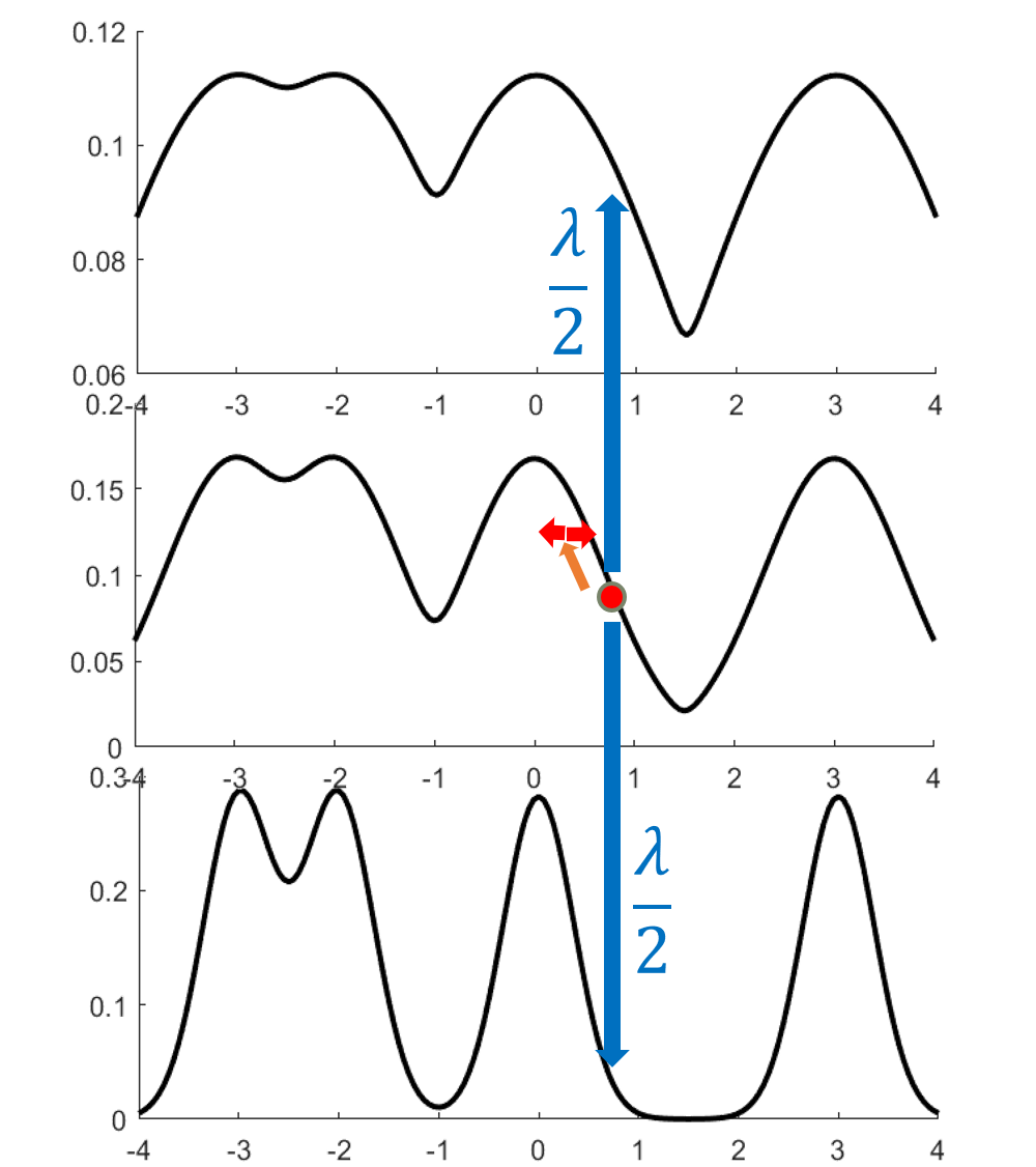
The main idea is to create a meta-Markov chain (the simulated tempering chain) which has two types of moves: change the current “temperature” of the sample, or move “within” a temperature. The main intuition behind this is that at higher temperatures, the distribution is flatter, so the chain explores the landscape faster (see the figure below).
More formally, the distribution at inverse temperature $\beta$ is given by $p_\beta(x) \propto e^{-\beta f(x)}$. The Langevin chain which corresponds to $\beta$ is given by
\[x_{t+\eta} = x_t - \eta \beta \nabla f(x_t) + \sqrt{2\eta}\xi_t,\quad \xi_t\sim N(0,I).\]As in the figure above, a high temperature (low $\beta<1$) flattens out the distribution and causes the chain to mix faster (top distribution in figure). However, we can’t merely run Langevin at a higher temperature, because the stationary distribution of the high-temperature chain is wrong: it’s $p_\beta(x)$. The idea behind simulated tempering is to run Langevin chains at different temperatures, sometimes swapping to another temperature to help lower-temperature chains explore. To maintain the right stationary distributions at each temperature, we use a Metropolis-Hastings filtering step.
More formally, choosing a suitable sequence $0< \beta_1< \cdots <\beta_L=1$, we define the simulated tempering chain as follows.
- The state space is a pair of a temperature and location in space $(i, x), i \in [L], x \in \mathbb{R}^d$.
- The transitions are defined as follows.
- If the current point is $(i,x)$, then evolve $x$ according to Langevin diffusion with inverse temperature $\beta_i$.
- Propose swaps with some rate $\lambda >0$. Proposing a swap means attempting to move to a neighboring chain, i.e. change $i$ to $i’=i\pm 1$. With probability $\min{p_{i’}(x)/p_i(x), 1}$, the transition is accepted. Otherwise, stay at the same point. This is a Metropolis-Hastings step; its purpose is to preserve the stationary distribution.
Finally, it’s not too hard to see that at the stationary distribution, the samples at the $L$th level ($\beta_L=1$) are the desired samples.
Proof idea: decomposition theorem
The main strategy is inspired by Madras and Randall’s Markov chain decomposition theorem, which gives a criterion for a Markov chain to mix rapidly: partition the state space into sets, and show that
- The Markov chain mixes rapidly when restricted to each set of the partition.
- The projected Markov Chain, which we define momentarily, mixes rapidly. If there are $m$ sets, the projected chain $\overline M$ is defined on the state space ${1,\ldots, m}$, and transition probabilities are given by average probability flows between the corresponding sets.
To implement this strategy, we first have to specify the partition. In fact, we roughly show that there is a partition of $[L] \times \mathbb{R}^d$ in which:
- The simulated tempering Langevin chain mixes fast within each of the sets.
- The “volume” of the sets (under the stationary distribution of the tempering chain) is not too small.
In applying the Madras-Randall framework with this partition, it’s clear that point (1) above satisfies requirement (1) for the framework; point (2) ensures that the projected Markov chain has no “bottlenecks” and hence that it mixes rapidly (requirement (2)). More precisely, we can show rapid mixing either through the method of canonical paths or Cheeger’s inequality. To do this, we exhibit a “good-probability” path between any two sets in the partition, going through the highest temperature.
The intuition for why this path works is illustrated in the figure below: when transitioning from the set corresponding to the left mode at level $L$ to the right mode at level $L$, each of the steps up/down the temperatures are accepted with good probability if the neighboring temperatures are not too different; at the highest temperature, the chain mixes fast by point (1), and since each of the sets are not too small by point (2), there is a reasonable probability to end at the right mode at the highest temperature.
Intuitively, the partition should track the “modes” of the distribution, but a technical hurdle in implementing this plan is in defining the partition when the modes overlap. One can either do this spectrally (i.e. showing that the Langevin chain has a spectral gap, and use theorems about spectral graph partitioning, as we did in the first version of the paper), or use a functional “soft decomposition theorem” which is a more flexible version of the classical decomposition theorem, which we use in a later version of the paper.