In the first post of this series, we introduced the challenges of sampling distributions beyond log-concavity. In Part 2 we tackled sampling from multimodal distributions: a typical obstacle occuring in problems involving statistical inference and posterior sampling in generative models. In this (final) post of the series, we consider sampling in the presence of manifold structure in the level sets of the distribution – which also frequently manifests in the same settings. It will cover the paper Fast convergence for Langevin diffusion with matrix manifold structure by Ankur Moitra and Andrej Risteski .

Sampling with matrix manifold structure

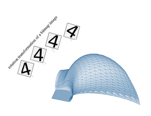
The structure on the distribution we consider in this post is manifolds of equiprobable points: this is natural, for instance, in the presence of invariances in data (e.g. rotations of images). It can also appear in neural-network based probabilistic models due to natural invariances they encode (e.g., scaling invariances in ReLU-based networks).

At the level of techniques, the starting point for our results is a close connection between the geometry, more precisely Ricci curvature of a manifold, and the mixing time of Brownian motion on a manifold. The following theorem holds:

Theorem (Bakry and Émery ‘85, informal): If the manifold $M$ has positive Ricci curvature, Brownian motion on the manifold mixes rapidly in $\chi^2$ divergence.

We will explain the notions from differential geometry shortly, but first we sketch our results, and how they use this machinery. We present two results: the first is a “meta”-theorem that provides a generic decomposition framework, and the second is an instantiation of this framework for a natural family of problems that exhibit manifold structure: posteriors for matrix factorization, sensing, and completion.

A general manifold decomposition framework

Our first result is a general decomposition framework for analyzing mixing time of Langevin in the presence of manifolds of equiprobable points.

To motivate the result, note that if we consider the distribution $p_{\beta}(x) \propto e^{-\beta f(x)}$, for large (but finite) $\beta$, the Langevin chain corresponding to that distribution, started close to a manifold of local minima, will tend to stay close to (but not on!) it for a long time. See the figure below for an illustration. This, we will state a “robust” version of the above manifold result, for a chain that’s allowed to go off the manifold.

We show the following statement. (Recall that a bounded Poincaré constant corresponds to rapid mixing for Langevin. See the first post for a refresher.)

Theorem 1 (Moitra and Risteski ‘20, informal): Suppose the Langevin chain corresponding to $p(x) \propto e^{-f(x)}$ is initialized close to a manifold $M$ satisfying the following two properties:

(1) It stays in some neighborhood $D$ of the manifold $M$ with large probability for a long time.

(2) $D$ can be partitioned into manifolds $M^{\Delta}$ satisfying:

(2.1) The conditional distribution of $p$ restricted to $M^{\Delta}$ has a upper bounded Poincare constant.

(2.2) The marginal distribution over $\Delta$ has a upper bounded Poincare constant.

(2.3) The conditional probability distribution over $M^{\Delta}$ does not “change too quickly” as $\Delta$ changes.

Then Langevin mixes quickly to a distribution close to the conditional distribution of $p$ restricted to $D$.

While the above theorem is a bit of a mouthful (even very informally stated) and requires a choice of partitioning of $D$ to be “instantiated”, it’s quite natural to think of it as an analogue of local convergence results for gradient descent in optimization. Namely, it gives geometric conditions under which Langevin started near a manifold mixes to the “local” stationary distribution (i.e. the conditional distribution $p$ restricted to $D$).

The proof of the theorem uses similar decomposition ideas as result on sampling multimodal distributions from the previous post, albeit is complicated by measure theoretic arguments. Namely, the manifolds $M^{\Delta}$ have technically zero measure under the distribution $p$, so care must be taken with how the “projected” and “restricted” chain are defined—the key tool for this is the so-called co-area formula.

The challenge in using the above framework is instantiating the decomposition: namely, the choice of the partition of $D$ into manifolds $M^{\Delta}$. In the next section, we show how this can be done for posteriors in problems like matrix factorization/sensing/completion.

Matrix factorization (and relatives)

To instantiate the above framework in a natural setting, we consider distributions exhibiting invariance under orthogonal transformations. Namely, we consider distributions of the type

where $b \in \mathbb{R}^{m}$ is a fixed vector and $\mathcal{A}$ is an operator that returns a $m$-dimensional vector given a $d \times d$ matrix. For this distribution, we have $p(X) = p(XO)$ for any orthogonal matrix $O$, since $XX^T = XO (XO)^T$ . Depending on the choice of $\mathcal{A}$, we can easily recover some familiar functions inside the exponential: e.g. the $l_2$ losses for (low-rank) matrix factorization, matrix sensing and matrix completion. These losses received a lot of attention as simple examples of objectives that are non-convex but can still be optimized using gradient descent. (See e.g. Ge et al. ‘17.)

These distributions also have a very natural statistical motivation. Namely, consider the distribution over $m$-dimensional vectors, such that

Then, the distribution $p(X) \propto e^{-\beta | \mathcal{A}(XX^T) - b |^2_2 }$ can be viewed as the posterior distribution over $X$ with a uniform prior. Thus, sampling from these distributions can be seen as the distributional analogue of problems like matrix factorization/sensing/completion, the difference being that we are not merely trying to find the most likely matrix $X$, but also trying to sample from the posterior.

We will consider the case when $\beta$ is sufficiently large (in particular, $\beta = \Omega(\mbox{poly}(d))$: in this case, the distribution $p$ will concentrate over two (separated) manifolds: $E_1 = \{X_0 R: R \mbox{ is orthogonal with det 1}\}$ and $E_2 = \{X_0 R: R \mbox{ is orthogonal with det }-1\}$, where $X_0$ is any fixed minimizer of $| \mathcal{A}(XX^T) - b |^2_2$. Hence, when started near one of these manifolds, we expect Langevin to stay close to it for a long time (see figure below).

We show:

Theorem 2 (Moitra and Risteski ‘20, informal): Let $\mathcal{A}$ correspond to matrix factorization, sensing or completion under standard parameter assumptions for these problems. Let $\beta = \Omega(\mbox{poly}(d))$. If initialized close to one of $E_i, i \in \{1, 2\}$, after a polynomial number of steps the discretized Langevin dynamics will converge to a distribution that is close in total variation distance to p(X) when restricted to a neighborhood of $E_i$.

We remark that the closeness condition for the first step is easy to ensure using existing results on gradient-descent based optimization for these objectives. It’s also easy to use the above result to sample approximately from the distribution $p$ itself, rather than only the “local” distributions $p^i$ – this is due to the fact that the distribution $p$ looks like the “disjoint union” of the distributions $p^1$ and $p^2$.

Before we describe the main elements of the proof, we review some concepts from differential geometry.

(Extremely) brief intro to differential geometry

We won’t do a full primer on differential geometry in this blog post, but we will briefly informally describe some of the relevant concepts. See Section 5 of our paper for an intro to differential geometry (written with a computer science reader in mind, so more easy-going than a differential geometry textbook).

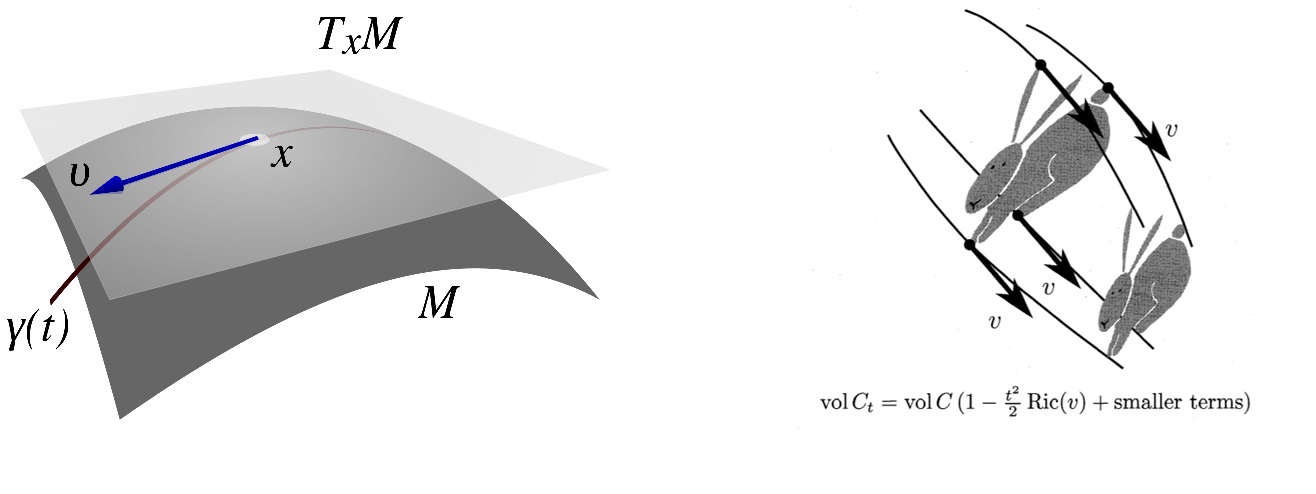
Recall, the tangent space at $x$, denoted by $T_x M$, is the set of all derivatives $v$ of a curve passing through $x$. The Ricci curvature at a point $x$, in direction $v \in T_x M$, denoted $\mbox{Ric}_x(v)$, captures the second-order term in the rate of change of volumes of sets in a small neighborhood around $x$, as the points in the set are moved along the geodesic (i.e. shortest path curve) in direction $v$ (or more precisely, each point $y$ in the set is moved along the geodesic in the direction of the parallel transport of $v$ at $y$; see the right part of the figure below from (Ollivier 2010)). A Ricci curvature of $0$ preserves volumes (think: a plane), a Ricci curvature $>0$ shrinks volume (think: a sphere), and a Ricci curvature $<0$ expands volume (think: a hyperbola).

The connections between curvature and mixing time of diffiusions is rather deep and we won’t attempt to convey it fully in a blog post - the definitive reference is Analysis and Geometry of Markov Diffusion Operators by Bakry, Gentil and Ledoux. The main idea is that mixing time can be bounded by how long it takes for random walks starting at different locations to “join together,” and positive curvature brings them together faster.

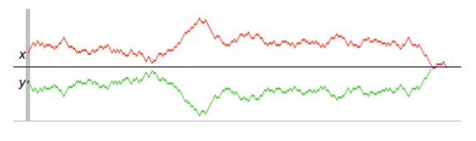
To make this formal, we define a coupling of two random variables $X, Y$ to be any random variable $W = (X’,Y’)$ such that the marginal distribution of the coordinates $X’$ and $Y’$ are the same as the distributions of $X$ and $Y$. It’s well known that the convergence time of a random walk in total variation distance can be upper bounded by the expected time until two coupled copies of the walk join. On the plane, a canonical coupling (the reflection coupling) between two Brownian motions can be constructed by reflecting the move of the second process through the perpendicular bisector between the locations of the two processes (see figure below). On a positively curved manifold (like a sphere), an analogous reflection can be defined, and the curvature only brings the two processes closer faster.

As a final tool, our proof uses a very important theorem due to Milnor about manifolds with algebraic structure:

Theorem (Milnor ‘76, informal): The Ricci curvature of a Lie group equipped with a left-invariant metric is non-negative.

In a pinch, a Lie group is a group that also is a smooth manifold, and furthermore, the group operations result in a smooth transformation on the manifold - so that the “geometry” and “algebra” combine together. A metric is left-invariant for the group if acting on the left by any group element leaves the metric “unchanged”.

Implementing the decomposition framework

To apply the framework we sketched out as part of Theorem 1, we need to verify the conditions of the Theorem.

To prove Condition 1, we need to show that for large $\beta$, the random walk stays near to the manifold it’s been initialized close to. The main tools for this are Ito’s lemma, local convexity of the function $| \mathcal{A}(XX^T) - b |_2^2$ and basic results in the theory of Cox-Ingersoll-Ross processes. Namely, Ito’s lemma (which can be viewed as a “change-of-variables” formula for random variables) allows us to write down a stochastic differential equation for the evolution of the distance of $X$ from the manifold, which turns out to have a “bias” towards small values, due to the local convexity of $| \mathcal{A}(XX^T) - b |_2^2$. This can in turn be analyzed approximately as Cox-Ingersoll-Ross process - a well-studied type of non-negative stochastic process.

To prove Condition 2, we need to specify the partition of the space around the manifolds $E_i$. Describing the full partition is somewhat technical, but importantly, the manifolds $M^{\Delta}$ have the form $M^{\Delta} = \{\Delta U: U \mbox{ is an orthogonal matrix with det 1}\}$ for some matrix $\Delta \in \mathbb{R}^{n \times k}$.

The proof that $M^{\Delta}$ has a good Poincare constant (i.e. Condition 2.1) relies on two ideas: first, $M^{\Delta}$ is a Lie group with group operation $\circ$ defined such that $(\Delta U) \circ (\Delta V) := \Delta (UV)$, along with a corresponding left-invariant metric - thus, by Milnor’s theorem, it has a non-negative Ricci curvature; second, we can relate the Ricci curvatures with the Euclidean metric to the curvature with the left-invariant metric. The proof that the marginal distribution over $\Delta$ has a good Poincaré constant involves showing that this distribution is approximately log-concave. Finally, the “change-of-conditional-probability” condition (Condition 2.3) can be proved by explicit calculation.

Closing remarks

In this series of posts, we surveyed two recent approaches to analyzing Langevin-like sampling algorithms beyond log-concavity - the most natural analogue to non-convexity in the world of sampling/inference. The structures we considered, multi-modality and invariant manifolds, are common in practice in modern machine learning.

Unlike non-convex optimization, provable guarantees for sampling beyond log-concavity is still under-studied and we hope our work will inspire and excite further efforts. For instance, how do we handle modes of different “shape”? Can we handle an exponential number of modes, if they have further structure (e.g., posteriors in concrete latent-variable models like Bayesian networks)? Can we handle more complex manifold structure (e.g. the matrix distributions we considered for any $\beta$)?