In effort to understand implicit regularization in deep learning, a lot of theoretical focus is being directed at matrix factorization, which can be seen as linear neural networks. This post is based on our recent paper (to appear at ICML 2021), where we take a step towards practical deep learning, by investigating tensor factorization — a model equivalent to a certain type of non-linear neural networks. It is well known that most tensor problems are NP-hard, and accordingly, the common sentiment is that working with tensors (in both theory and practice) entails extreme difficulties. However, by adopting a dynamical systems view, we manage to avoid such difficulties, and establish an implicit regularization towards low tensor rank. Our results suggest that tensor rank may shed light on generalization in deep learning.
Challenge: finding a right measure of complexity
Overparameterized neural networks are mysteriously able to generalize even when trained without any explicit regularization. Per conventional wisdom, this generalization stems from an implicit regularization — a tendency of gradient-based optimization to fit training examples with predictors of minimal ‘‘complexity.’’ A major challenge in translating this intuition to provable guarantees is that we lack measures for predictor complexity that are quantitative (admit generalization bounds), and at the same time, capture the essence of natural data (images, audio, text etc.), in the sense that it can be fit with predictors of low complexity.
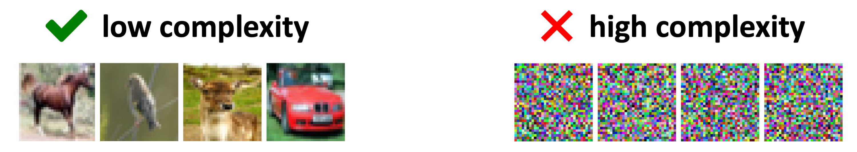
Figure 1: To explain generalization in deep learning, a complexity
measure must allow the fit of natural data with low complexity. On the
other hand, when fitting data which does not admit generalization,
e.g. random data, the complexity should be high.
A common testbed: matrix factorization
Without a clear complexity measure for practical neural networks, existing analyses usually focus on simple settings where a notion of complexity is obvious. A common example of such a setting is matrix factorization — matrix completion via linear neural networks. This model was discussed pretty extensively in previous posts (see one by Sanjeev, one by Nadav and Wei and another one by Nadav), but for completeness we present it again here.
In matrix completion we’re given a subset of entries from an unknown matrix $W^* \in \mathbb{R}^{d, d’}$, and our goal is to predict the unobserved entries. This can be viewed as a supervised learning problem with $2$-dimensional inputs, where the label of the input $( i , j )$ is $( W^* )_{i,j}$. Under such a viewpoint, the observed entries are the training set, and the average reconstruction error over unobserved entries is the test error, quantifying generalization. A predictor can then be thought of as a matrix, and a natural notion of complexity is its rank. Indeed, in many real-world scenarios (a famous example is the Netflix Prize) one is interested in recovering a low rank matrix from incomplete observations.
A ‘‘deep learning approach’’ to matrix completion is matrix factorization, where the idea is to use a linear neural network (fully connected neural network with no non-linearity), and fit observations via gradient descent (GD). This amounts to optimizing the following objective:
It is obviously possible to constrain the rank of the produced solution by limiting the shared dimensions of the weight matrices $\{ W_j \}_j$. However, from an implicit regularization standpoint, the most interesting case is where rank is unconstrained and the factorization can express any matrix. In this case there is no explicit regularization, and the kind of solution we get is determined implicitly by the parameterization and the optimization algorithm.
As it turns out, in practice, matrix factorization with near-zero initialization and small step size tends to accurately recover low rank matrices. This phenomenon (first identified in Gunasekar et al. 2017) manifests some kind of implicit regularization, whose mathematical characterization drew a lot of interest. It was initially conjectured that matrix factorization implicitly minimizes nuclear norm (Gunasekar et al. 2017), but recent evidence points to implicit rank minimization, stemming from incremental learning dynamics (see Arora et al. 2019; Razin & Cohen 2020; Li et al. 2021). Today, it seems we have a relatively firm understanding of generalization in matrix factorization. There is a complexity measure for predictors — matrix rank — by which implicit regularization strives to lower complexity, and the data itself is of low complexity (i.e. can be fit with low complexity). Jointly, these two conditions lead to generalization.
Beyond matrix factorization: tensor factorization
Matrix factorization is interesting on its own behalf, but as a theoretical surrogate for deep learning it is limited. First, it corresponds to linear neural networks, and thus misses the crucial aspect of non-linearity. Second, viewing matrix completion as a prediction problem, it doesn’t capture tasks with more than two input variables. As we now discuss, both of these limitations can be lifted if instead of matrices one considers tensors.
A tensor can be thought of as a multi-dimensional array. The number of axes in a tensor is called its order. In the task of tensor completion, a subset of entries from an unknown tensor $\mathcal{W}^* \in \mathbb{R}^{d_1, \ldots, d_N}$ are given, and the goal is to predict the unobserved entries. Analogously to how matrix completion can be viewed as a prediction problem over two input variables, order-$N$ tensor completion can be seen as a prediction problem over $N$ input variables (each corresponding to a different axis). In fact, any multi-dimensional prediction task with discrete inputs and scalar output can be formulated as a tensor completion problem. Consider for example the MNIST dataset, and for simplicity assume that image pixels hold one of two values, i.e. are either black or white. The task of predicting labels for the $28$-by-$28$ binary images can be seen as an order-$784$ (one axis for each pixel) tensor completion problem, where all axes are of length $2$ (corresponding to the number of values a pixel can take). For further details on how general prediction tasks map to tensor completion problems see our paper.
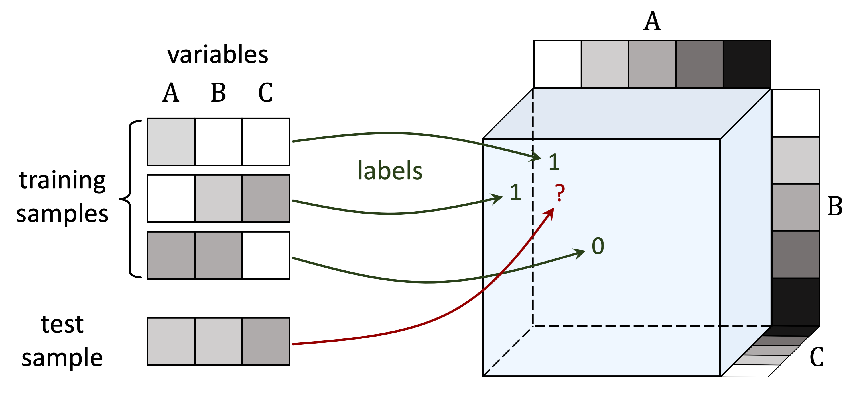
Figure 2: Prediction tasks can be viewed as tensor completion problems.
For example, predicting labels for input images with $3$ pixels, each taking
one of $5$ grayscale values, corresponds to completing a $5 \times 5 \times 5$ tensor.
Like matrices, tensors can be factorized.
The most basic scheme for factorizing tensors, named CANDECOMP/PARAFAC (CP), parameterizes a tensor as a sum of outer products (for information on this scheme, as well as others, see the excellent survey of Kolda and Bader).
In our paper and this post, we use the term tensor factorization to refer to solving tensor completion by fitting observations via GD over CP parameterization, i.e. over the following objective ($\otimes$ here stands for outer product):
The concept of rank naturally extends from matrices to tensors. The tensor rank of a given tensor $\mathcal{W}$ is defined to be the minimal number of components (i.e. of outer product summands) $R$ required for CP parameterization to express it. Note that for order-$2$ tensors, i.e. for matrices, this exactly coincides with matrix rank. We can explicitly constrain the tensor rank of solutions found by tensor factorization via limiting the number of components $R$. However, since our interest lies on implicit regularization, we consider the case where $R$ is large enough for any tensor to be expressed.
By now you might be wondering what does tensor factorization have to do with deep learning. Apparently, as Nadav mentioned in an earlier post, analogously to how matrix factorization is equivalent to matrix completion (two-dimensional prediction) via linear neural networks, tensor factorization is equivalent to tensor completion (multi-dimensional prediction) with a certain type of non-linear neural networks (for the exact details behind the latter equivalence see our paper). It therefore represents a setting one step closer to practical neural networks.
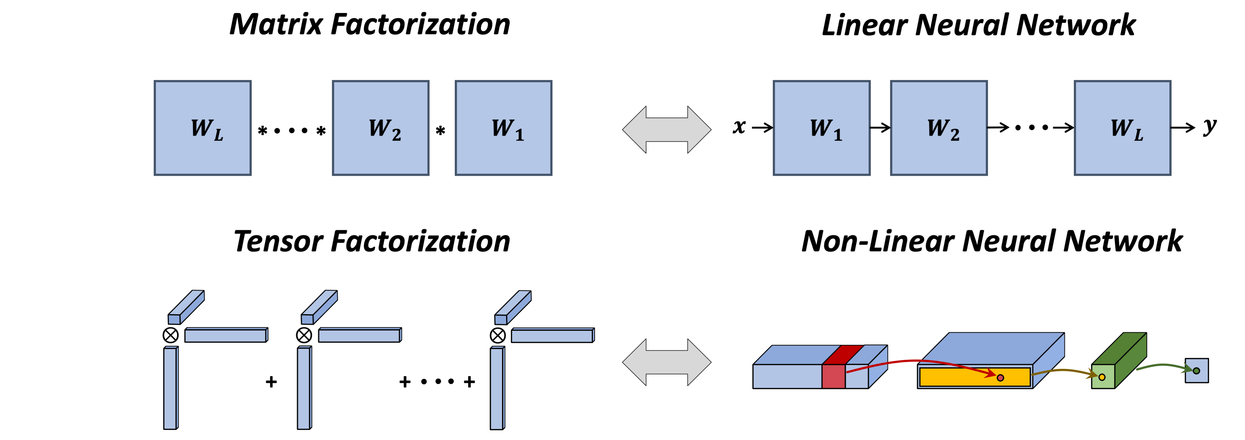
Figure 3: While matrix factorization corresponds to a linear neural network,
tensor factorization corresponds to a certain non-linear neural network.
As a final piece of the analogy between matrix and tensor factorizations, in a previous paper (described in an earlier post) Noam and Nadav demonstrated empirically that (similarly to the phenomenon discussed above for matrices) tensor factorization with near-zero initialization and small step size tends to accurately recover low rank tensors.
Our goal in the current paper was to mathematically explain this finding.
To avoid the notorious difficulty of tensor problems, we chose to adopt a dynamical systems view, and analyze directly the trajectories induced by GD.
Dynamical analysis: implicit tensor rank minimization
So what can we say about the implicit regularization in tensor factorization? At the core of our analysis is the following dynamical characterization of component norms:
Theorem: Running gradient flow (GD with infinitesimal step size) over a tensor factorization with near-zero initialization leads component norms to evolve by: [ \frac{d}{dt} || \mathbf{w}_r^1 (t) \otimes \cdots \otimes \mathbf{w}_r^N (t) || \propto \color{brown}{|| \mathbf{w}_r^1 (t) \otimes \cdots \otimes \mathbf{w}_r^N (t) ||^{2 - 2/N}} ~, ] where $\mathbf{w}_r^1 (t), \ldots, \mathbf{w}_r^N (t)$ denote the weight vectors at time $t \geq 0$.
According to the theorem above, component norms evolve at a rate proportional to their size exponentiated by $\color{brown}{2 - 2 / N}$ (recall that $N$ is the order of the tensor to complete). Consequently, they are subject to a momentum-like effect, by which they move slower when small and faster when large. This suggests that when initialized near zero, components tend to remain close to the origin, and then, after passing a critical threshold, quickly grow until convergence. Intuitively, these dynamics induce an incremental process where components are learned one after the other, leading to solutions with a few large components and many small ones, i.e. to (approximately) low tensor rank solutions!
We empirically verified the incremental learning of components in many settings. Here is a representative example from one of our experiments (see the paper for more):
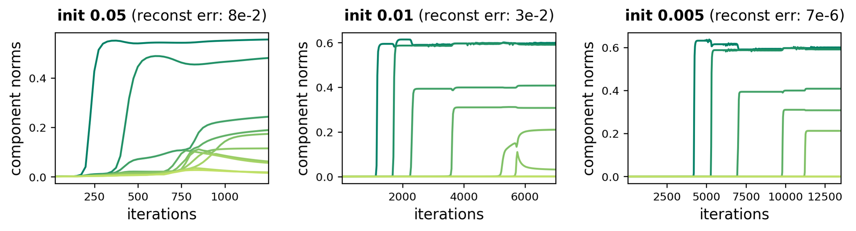
Figure 4: Dynamics of component norms during GD over tensor factorization.
An incremental learning effect is enhanced as initialization scale decreases,
leading to accurate completion of a low rank tensor.
Using our dynamical characterization of component norms, we were able to prove that with sufficiently small initialization, tensor factorization (approximately) follows a trajectory of rank one tensors for an arbitrary amount of time.
This leads to:
Theorem: If tensor completion has a rank one solution, then under certain technical conditions, tensor factorization will reach it.
It’s worth mentioning that, in a way, our results extend to tensor factorization the incremental rank learning dynamics known for matrix factorization (cf. Arora et al. 2019 and Li et al. 2021). As typical when transitioning from matrices to tensors, this extension entailed various challenges that necessitated use of different techniques.
Tensor rank as measure of complexity
Going back to the beginning of the post, recall that a major challenge towards understanding implicit regularization in deep learning is that we lack measures for predictor complexity that capture natural data. Now, let us recap what we have seen thus far: $(1)$ tensor completion is equivalent to multi-dimensional prediction; $(2)$ tensor factorization corresponds to solving the prediction task with certain non-linear neural networks; and $(3)$ the implicit regularization of these non-linear networks, i.e. of tensor factorization, minimizes tensor rank. Motivated by these findings, we ask the following:
Question: Can tensor rank serve as a measure of predictor complexity?
We empirically explored this prospect by evaluating the extent to which tensor rank captures natural data, i.e. to which natural data can be fit with predictors of low tensor rank. As testbeds we used MNIST and Fashion-MNIST datasets, comparing the resulting errors against those obtained when fitting two randomized variants: one generated via shuffling labels (‘‘rand label’’), and the other by replacing inputs with noise (‘‘rand image’’).
The following plot, displaying results for Fashion-MNIST (those for MNIST are similar), shows that with predictors of low tensor rank the original data is fit way more accurately than the randomized datasets. Specifically, even with tensor rank as low as one the original data is fit relatively well, while the error in fitting random data is close to trivial (variance of the label). This suggests that tensor rank as a measure of predictor complexity has potential to capture aspects of natural data! Note also that an accurate fit with low tensor rank coincides with low test error, which is not surprising given that low tensor rank predictors can be described with a small number of parameters.
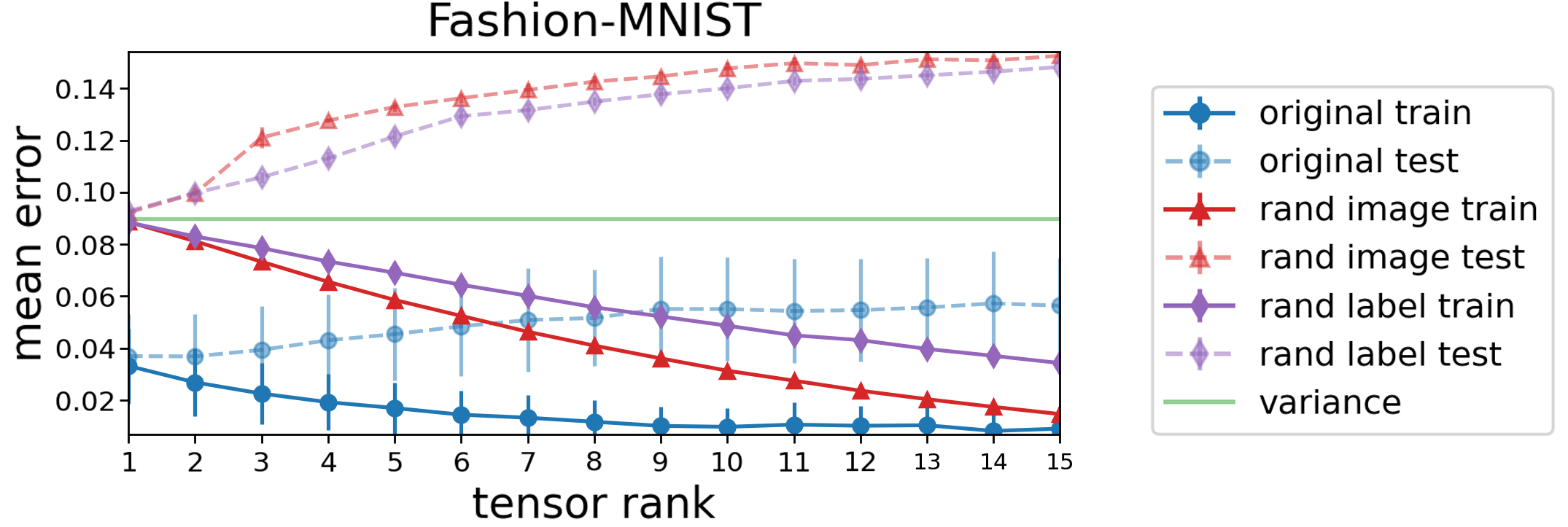
Figure 5: Evaluation of tensor rank as a measure of complexity — standard datasets
can be fit accurately with predictors of low tensor rank (far beneath what is required by
random datasets), suggesting it may capture aspects of natural data. Plot shows mean
error of predictors with low tensor rank over Fashion-MNIST. Markers correspond
to separate runs differing in the explicit constraint on the tensor rank.
Concluding thoughts
Overall, our paper shows that tensor rank captures both the implicit regularization of a certain type of non-linear neural networks, and aspects of natural data. In light of this, we believe tensor rank (or more advanced notions such as hierarchical tensor rank) might pave way to explaining both implicit regularization in more practical neural networks, and the properties of real-world data translating this implicit regularization to generalization.